Molecular Docking studies
Author: Juan Pablo Cerutti (jpcerutti@unc.edu.ar) – September 2025
Aminoglycosides
Aminoglycosides are natural or semisynthetic, potent, broad-spectrum antimicrobials active mainly against aerobic organisms, including gram-negative bacteria and mycobacteria. This class has been a cornerstone of antibacterial chemotherapy since streptomycin was first isolated from Streptomyces griseus and introduced into clinical practice in 1944. Over the following decades, several other members were developed, including neomycin (1949, S. fradiae), kanamycin (1957, S. kanamyceticus), gentamicin (1963, Micromonospora purpurea), and tobramycin (1967, S. tenebrarius). Their medical relevance is such that they are included in the WHO list of medically important antimicrobials for human medicine.1,2,3
Mechanistically, aminoglycosides exert bactericidal activity by binding to the bacterial ribosomal 30S subunit, specifically to the A-site (aminoacyl) of the 16S rRNA. This interaction induces codon misreading and disrupts translation, ultimately blocking protein synthesis. Owing to the structural differences between prokaryotic and eukaryotic ribosomes, aminoglycosides are selective drugs; however, they are associated with nephrotoxic and ototoxic side effects. Ototoxicity has been reported in 2–45% of adults, while nephrotoxicity occurs in up to 10–25% of patients. The availability of third-generation cephalosporins, carbapenems, and fluoroquinolones in the 1980s reduced systemic use of aminoglycosides, but the rise of multidrug-resistant (MDR) pathogens has renewed interest in this antibiotic class.1,2,3
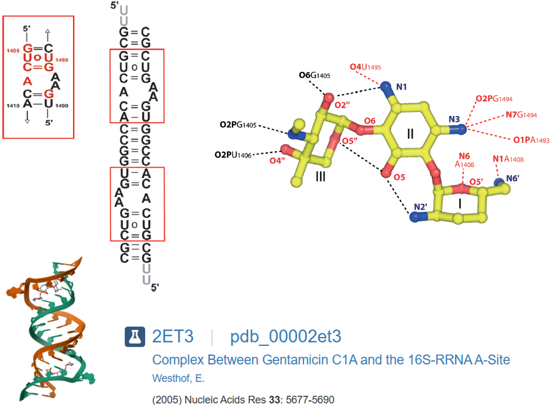
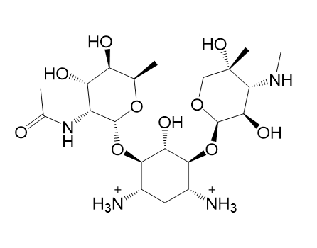
Structurally, aminoglycosides are based on aminocyclitol aglycones such as 2-deoxystreptamine (2-DOS), streptamine, or streptidine. The most active compounds typically contain 2-DOS as the aglycone unit, including gentamicin.1,2,3 Gentamicin remains clinically important for treating sinopulmonary infections (notably in cystic fibrosis), complicated urinary tract infections, and as empiric therapy in neonates. Its use is, however, limited by reversible nephrotoxicity and irreversible ototoxicity. Gentamicin is also distinctive in that it is supplied as a mixture of major and minor components rather than as a single, well-defined structure (Figure 1). According to the U.S. Pharmacopeia (USP), formulations must contain 10–35% gentamicin C1a, 25–55% gentamicin C2/C2a, and 25–50% gentamicin C1. This variability implies that antibacterial activity can differ across USP-compliant products.

Recent studies have systematically examined the antimicrobial activity and ototoxicity of individual gentamicin components, including minor congeners and impurities.2 Results showed that the five major congeners (C1, C1a, C2, C2a, C2b) and the minor component sisomicin were as potent as the mixture, indicating that the broad spectrum of gentamicin is not due to being a mixture. Importantly, only C2b displayed lower ototoxicity than the mixture; C1, C1a, and C2a showed comparable toxicity, while C2 and several “impurities” were more toxic. Despite these insights, no clear structure–activity relationships (SAR) were defined to rationalize potency differences among congeners. Such knowledge would be valuable for designing safer, more potent gentamicin analogues.
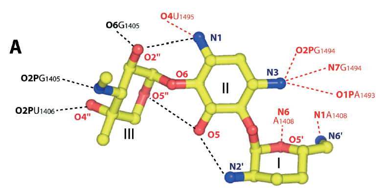
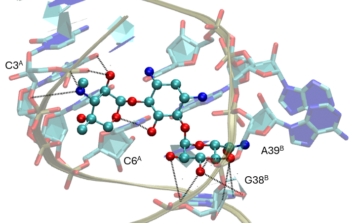
Crystallographic structures of gentamicin C1a bound to the ribosomal A-site (PDB ID: 2ET3) provide an excellent starting point for molecular docking, since they capture the antibiotic in complex with its physiological target (Figure 2), enabling validation of docking protocols and serving as a reference to assess the reliability of predicted binding modes for other congeners.
Thus, in this tutorial we will:
- Replicate the crystallographic binding mode Gentamicin C1a to validate the target and define appropriate docking conditions.
- Extend the study to the full set of gentamicin congeners (major and minor) to explore potential pharmacodynamic bases for the reported differences in potency.
- Perform docking-based virtual high-throughput screening (vHTS) to identify novel gentamicin analogues as promising candidates with improved antimicrobial activity.
In this tutorial, we will rely on the following software packages:
- AutoDock for the molecular docking studies.
- AutoDock Tools (ADT) to prepare receptors, ligands, grid parameters and other files required by AutoDock.
- Open Babel for format conversion and ligand preprocessing.
- ProLIF and MMGBSA for post-docking interaction fingerprint analysis and energetic decomposition.
For further guidance on installation, parameters, or advanced usage, please consult the official documentation and tutorials of each package.
1. Replication of the crystallographic binding mode of Gentamicin
Create and activate a dedicated TidyScreen project to store, process, filter and synthesize the target library of compounds:
# Import required modules
from tidyscreen import tidyscreen as ts
from tidyscreen.chemspace import chemspace as chemspace
from tidyscreen.moldock import moldock as moldock
from tidyscreen.docking_analysis import docking_analysis as docking_analysis
from tidyscreen.GeneralFunctions import general_functions as general_functions

# Create a dedicated project for the synthesis
ts.create_project("$HOME/Desktop/example", "Aminoglycosides")

# Activate the project just created
Aminoglycosides_example = ts.ActivateProject("Aminoglycosides")
The first step in the study involves the replication of the crystallographic complex. For this purpose, the target RNA helix and the gentamicin C1a ligand must be parametrized so that their experimental structural data can be converted into appropriate docking inputs. This parametrization ensures consistency with the crystallographic reference and allows a rigorous assessment of the docking protocol.
Molecular docking software requires both the receptor (target) and the ligand to be converted into simplified, parameterized formats that define atom types, charges, torsions, and connectivity.
This step ensures that the experimentally solved crystal structure can be translated into a computational model compatible with docking engines. Without proper parametrization, the docking algorithm may fail to recognize key interactions or generate unrealistic binding poses.
In particular, AutoDock requires .pdbqt files.
1.1. Receptor preparation
1.1.1. Download, clean and parametrize the crystal
The first step consists of preparing the RNA target from the crystallographic structure (PDB ID: 2ET3) so that it can be used by AutoDock.
This involves downloading the structure, removing non-essential molecules (ligand, solvent, crystallization agents), adding hydrogens at physiological pH, and finally generating a parameterized .pdbqt file with the correct atom types and charges.
Thus, inside the $HOME/Desktop/example/Aminoglycosides/docking/raw_data folder (which is automatically generated during project creation), run the following script:
# Create a new folder
mkdir genta_target && cd genta_target

# Download PDB
wget https://files.rcsb.org/download/2ET3.pdb

# Remove any HETATM (ligand, solvent, etc.) to isolate the target.
pdb_delhetatm 2ET3.pdb > genta_target.pdb

# Select one of the crystal structures of gentamicin C1a to keep as reference.
pdb_selresname -LLL 2ET3.pdb | pdb_selchain -B > genta.pdb

# Open Babel to add H at pH ~7.4
obabel -ipdb genta_target.pdb -opdb -p 7.4 -O genta_target.pdb

# Generate PDBQT files
# NOTE: `prepare_receptor4.py` and `prepare_ligand4.py` are provided within AutoDockTools (MGLTools).
# Replace /PATH/TO/MGLTOOLS with the path where MGLTools was installed on your system.
# Example: $HOME/mgltools_x86_64Linux2_1.5.7/bin/pythonsh

/PATH/TO/MGLTOOLS/bin/pythonsh prepare_receptor4.py -r genta_target.pdb -o genta_target.pdbqt -A checkhydrogens -U nphs_lps_waters

/PATH/TO/MGLTOOLS/bin/pythonsh prepare_ligand4.py -l genta.pdb -A hydrogens
You should get two new files: genta_target.pdbqt and genta.pdbqt.
1.1.2. Grid box
Define a grid box centered on the crystallographic ligand (A-site) and generate AutoGrid maps for AutoDock4.
Using python, run the following code to get the grid center of the aminoglycosides binding site.
import sys, re
fn = sys.argv[1] if len(sys.argv)>1 else 'genta.pdb'
xs,ys,zs,n=0.0,0.0,0.0,0
pat = re.compile(r'^(ATOM  |HETATM)')
with open(fn) as f:
    for line in f:
        if pat.match(line):
            try:
                x=float(line[30:38]); y=float(line[38:46]); z=float(line[46:54])
                xs+=x; ys+=y; zs+=z; n+=1
            except: pass

print(f"center_x={xs/n:.3f} center_y={ys/n:.3f} center_z={zs/n:.3f}")
you should get an output similar to the following:
center_x=31.474 center_y=7.643 center_z=26.304
Now, we define the Grid Parameter File (GPF) to generate the AutoGrid maps.
/PATH/TO/MGLTOOLS/bin/pythonsh prepare_gpf4.py -l genta.pdbqt -r genta_target.pdbqt -p npts=64,48,50 -p spacing=0.300 -p ligand_types=C,HD,OA,N,NA -p gridcenter=31.474,7.643,26.304
The genta_target.gpf file should be created.
npts 64 48 50                        # num.grid points in xyz
gridfld genta_target.maps.fld        # grid_data_file
spacing 0.300                        # spacing(A)
receptor_types A C NA OA N P HD      # receptor atom types
ligand_types C HD OA N NA            # ligand atom types
receptor genta_target.pdbqt          # macromolecule
gridcenter 31.474 7.643 26.304       # xyz-coordinates or auto
smooth 0.5                           # store minimum energy w/in rad(A)
map genta_target.C.map               # atom-specific affinity map
map genta_target.HD.map              # atom-specific affinity map
map genta_target.OA.map              # atom-specific affinity map
map genta_target.N.map               # atom-specific affinity map
map genta_target.NA.map              # atom-specific affinity map
elecmap genta_target.e.map           # electrostatic potential map
dsolvmap genta_target.d.map          # desolvation potential map
dielectric -0.1465                   # <0, AD4 distance-dep.diel;>0, constant
With the grid parameter file prepared, the next step is to run AutoGrid.
This program uses the receptor and the defined grid box to generate the energy maps required by AutoDock4.
These maps describe the interaction potentials of the ligand atom types within the receptor binding site and are essential for the subsequent docking step.
autogrid4 -p genta_target.gpf
After completion, AutoGrid will produce:
-
One .map file per ligand atom type (
genta_target.C.map,genta_target.HD.map,genta_target.N.map,genta_target.NA.map,genta_target.OA.map,genta_target.d.map,genta_target.e.map). -
A .fld file (
genta_target.maps.fld) that collects all maps.
# AVS field file
# AutoDock Atomic Affinity and Electrostatic Grids
# Created by autogrid4.
#
#SPACING 0.300
#NELEMENTS 64 48 50
#CENTER 31.474 7.643 26.304
#MACROMOLECULE genta_target.pdbqt
#GRID_PARAMETER_FILE genta_target.gpf
#
ndim=3			# number of dimensions in the field
dim1=65			# number of x-elements
dim2=49			# number of y-elements
dim3=51			# number of z-elements
nspace=3		# number of physical coordinates per point
veclen=7		# number of affinity values at each point
data=float		# data type (byte, integer, float, double)
field=uniform		# field type (uniform, rectilinear, irregular)
coord 1 file=genta_target.maps.xyz filetype=ascii offset=0
coord 2 file=genta_target.maps.xyz filetype=ascii offset=2
coord 3 file=genta_target.maps.xyz filetype=ascii offset=4
label=C-affinity	# component label for variable 1
label=HD-affinity	# component label for variable 2
label=OA-affinity	# component label for variable 3
label=N-affinity	# component label for variable 4
label=NA-affinity	# component label for variable 5
label=Electrostatics	# component label for variable 5
label=Desolvation	# component label for variable 6
#
# location of affinity grid files and how to read them
#
variable 1 file=genta_target.C.map filetype=ascii skip=6
variable 2 file=genta_target.HD.map filetype=ascii skip=6
variable 3 file=genta_target.OA.map filetype=ascii skip=6
variable 4 file=genta_target.N.map filetype=ascii skip=6
variable 5 file=genta_target.NA.map filetype=ascii skip=6
variable 6 file=genta_target.e.map filetype=ascii skip=6
variable 7 file=genta_target.d.map filetype=ascii skip=6
1.2. Ligand: Gentamicin C1a
In order to replicate the crystal structure, we will run docking studies with Gentamicin C1a and the receptor we just parametrized.
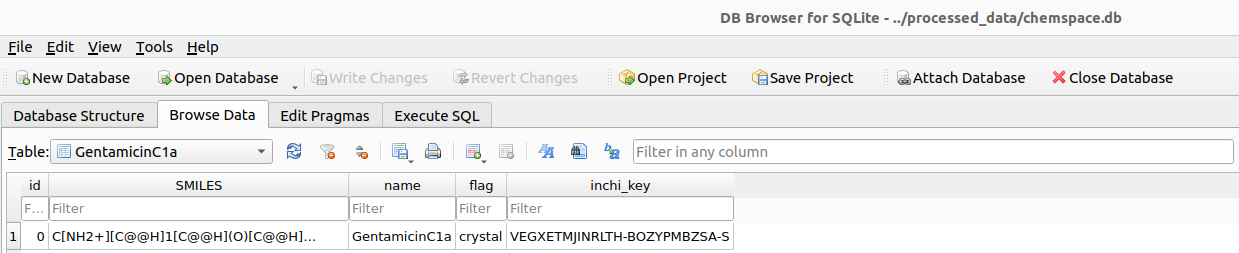
To do that, in the $HOME/Desktop/example/Aminoglycosides/chemspace/raw_data/ create a file called GentamicinC1a.csv containing the SMILES of the ligand.
CN[C@@H]3[C@@H](O)[C@@H](O[C@H]2[C@H]([NH3+])C[C@H]([NH3+])[C@@H](O[C@H]1O[C@H](C[NH3+])CC[C@H]1[NH3+])[C@@H]2O)OC[C@]3(C)O,GentamicinC1a,2ET3
Then, activate the chemspace module within Aminoglycosides.py.
# Activate the ChemSpace section of the project
aminoglycosides_example_chemspace = chemspace.ChemSpace(Aminoglycosides_example)

# Import the .csv file
aminoglycosides_example_chemspace.input_csv("$HOME/Desktop/example/Aminoglycosides/chemspace/raw_data/GentamicinC1a.csv")
After preparing the receptor, the next step is to generate the ligand files required for docking.
Specifically, we need to obtain both .pdb and .pdbqt formats for AutoDock.
Since these molecules may also be subjected to molecular dynamics simulations later on, we will additionally generate .mol2 and .frcmod files.
Atomic charges are assigned using EspalomaCharge, which provides accurate parameterization compatible with docking and dynamics workflows.
# Parametrization
aminoglycosides_example_chemspace.generate_mols_in_table("GentamicinC1a", timeout=1000)
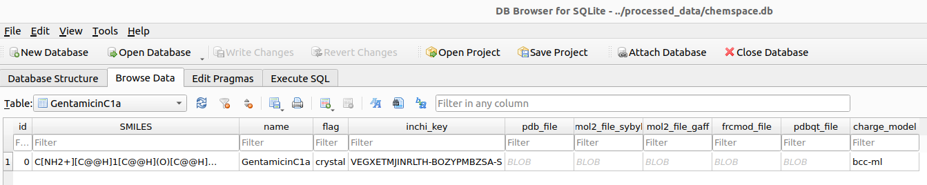
.pdb, .pdbqt, .mol2, and .frcmod) after parameterization. At this stage, all the necessary input files have been prepared, and we are ready to proceed with the docking study.
1.3. First docking validation
In order to validate our docking protocol, the first step is to compare the predicted binding pose with the crystallographic reference to evaluate whether the chosen docking parameters (grid size, spacing, scoring function, and search algorithm) are able to reproduce the native interaction mode. A successful docking provides confidence that the protocol is suitable to be extended to other congeners and to virtual screening campaigns.
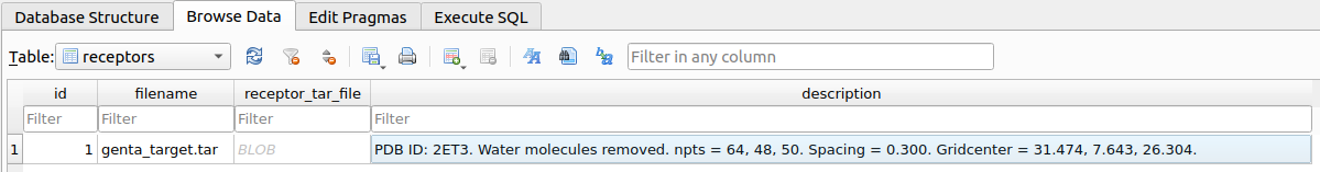
To proceed, we first activate the moldock module from TidyScreen and register the prepared receptor by creating a database entry that points to the target files (.map grids, .pdbqt, .fld, and reference .pdb).
# Initialize MolDock
aminoglycosides_example_docking = moldock.MolDock(Aminoglycosides_example)

# Register the receptor in the database, indicating the path to the folder containing the receptor/grid files.
aminoglycosides_example_docking.input_receptor("$HOME/Desktop/example/Aminoglycosides/docking/raw_data/genta_target")
When prompted, you will need to provide a short description of the receptor.
Try to include as many relevant details as possible, such as:
- PDB ID
- Preprocessing (waters/ions removed, protonation state)
- Grid setup (center, npts, spacing)
- Any special considerations (e.g. retained Mg²⁺)
This information will be very useful in the future, especially when your database grows and you manage multiple receptor models.
docking/receptors/receptor.db. Before running the docking experiment, it is necessary to define the docking parameters.
The function create_docking_params_set() generates a database (docking/params/docking_params.db) containing the default AutoDock conditions.
aminoglycosides_example_docking.create_docking_params_set()

docking/params/docking_params.db. Once the default set has been created, you may duplicate and customize the conditions to better suit your study. For example, you can increase the number of docking runs from 20 to 100 (--nrun=100) or enable AutoDock to identify and report ligand–receptor interactions for each pose (--contact_analysis=1).
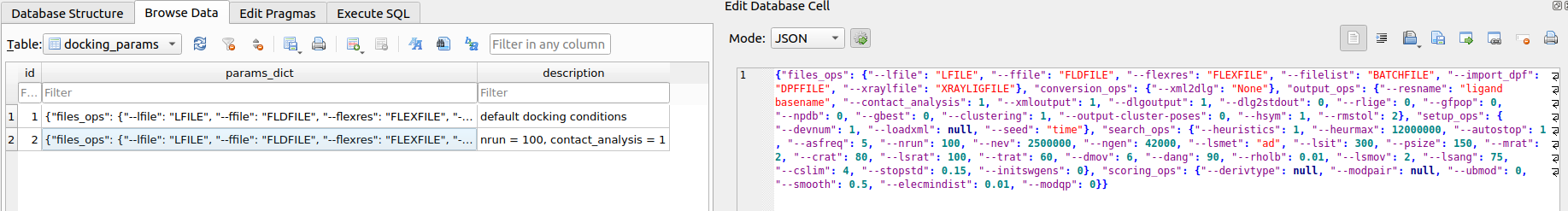
docking/params/docking_params.db. Now we can launch the docking experiment with the dock_table() function.
TidyScreen prepares all required input files and executes the docking through AutoDock-GPU, the GPU-accelerated implementation of AutoDock4. This allows a substantial speed-up compared to the CPU version, while maintaining compatibility with the same scoring function and parameter set.
You must define 3 variables:
- table_name: name of the table containing the ligand(s) you want to use for the docking study, as stated in the
chemspace/processed_data/chemspace.dbdatabase. - id_receptor_model: ID of the target model you want to use for the docking study, as stated in the
docking/receptors/receptor.dbdatabase. - id_docking_params: ID of the docking conditions you want to apply for the study, as stated in the
docking/params/docking_params.dbdatabase.
Once again you will be asked to provide a brief description of the docking assay. Try to include as many relevant details as possible.
Make sure that the IDs (id_receptor_model and id_docking_params) correspond to the entries you created earlier. If in doubt, you can query the databases to list available IDs before running the docking.
aminoglycosides_example_docking.dock_table(table_name="GentamicinC1a", id_receptor_model=1, id_docking_params=2)
After running dock_table(), TidyScreen will:
- Create a summary entry of the assay (variables + description) in
docking/docking_registers/docking_registers.db. - Create a new assay folder under
docking/docking_assays/assay_<ASSAY_ID>containing:- receptor/ and ligands/ subfolders with all input files,
- a ready-to-run execution script:
docking_execution.sh.
You can launch the assay in your terminal with:
./docking_execution.sh
1.4. Inspecting AutoDock outputs
After execution, AutoDock produces a docking log (.dlg) for each ligand under: docking/docking_assays/assay_<ASSAY_ID>/dlgs/.
Each .dlg file summarizes:
- the predicted poses (coordinates),
- the interaction report per pose (if
--contact_analysis=1), - the docking score (binding energy) of each conformation,
- and a cluster size summary at the end of the file.
The cluster size indicates how many independent runs converged to (approximately) the same pose.
For example, if --nrun=100 and a cluster reports size = 80, it means 80/100 runs found that pose as the best (lowest energy) within that cluster. Larger clusters often suggest higher pose stability/reproducibility under the search settings.

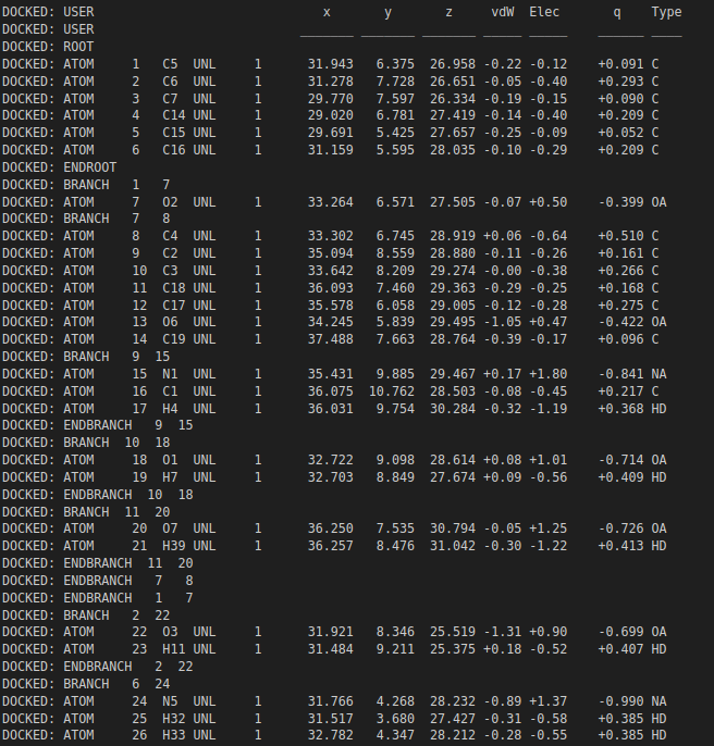
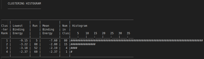
.dlg file. Top: docking scores and list of detected interactions. Middle: coordinates of a docked pose. Bottom: clustering histogram showing how many times each pose was identified during multiple runs. 1.5. Docking analyses
1.5.1. Autodock output
In this first example, analysing the .dlg file and the docked poses is relatively straightforward, since the study involved only a single ligand. However, when working with larger ligand sets, manual inspection quickly becomes impractical. For this reason, TidyScreen provides a DockingAnalysis module and a process_docking_assay() function to automate the post-processing of docking results.
When activating the DockingAnalysis module, you can specify the path to AMBER (via amberhome).
This way, the program will automatically use this path during the analyses, instead of prompting you for it every time you run a single analysis.
#Activate the module
aminoglycosides_example_docking_analysis = docking_analysis.DockingAnalysis(Aminoglycosides_example, amberhome="/PATH/TO/AMBER/amber<VERSION>")
The process_docking_assay() function parses the AutoDock outputs of a given assay, leveraging the Ringtail library to efficiently handle the results. It ranks the poses by docking score (most negative = best) and stores the selected results for downstream analysis.
You should define the following variables:
- assay_id (int, required): ID of the docking assay to analyze (as registered by dock_table()).
- max_poses (int, default = 10): Maximum number of poses per ligand to store in the results database, ordered from best (lowest binding energy) to worse.
- vmd_path (str | None, default = None): Path to VMD (Visual Molecular Dynamics). If provided, helper files/commands for quick visualization are prepared.
- extract_poses (int [0,1], default = 0): If 1, writes PDB files for each selected pose. If 0, keeps only the database records and existing PDBQT/DLG outputs.
#Set and run the docking analysis
aminoglycosides_example_docking_analysis.process_docking_assay(assay_id=1, max_poses=10, vmd_path="PATH/TO/VMD", extract_poses=1)
As a result, a new database assay_<ID>.db will be generated inside the corresponding assay docking folder.
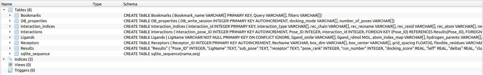
This file contains several tables that organize the results of the analysis:
-
interaction_indices: dictionary of interaction types (e.g., hydrogen bonds H and van der Waals V) that can be identified between ligands and receptor.
-
interactions: records which interactions were detected for each docked pose of every ligand.
-
ligands: stores ligand-specific data and a summary of their detected interactions.
-
receptor: summary information of the target used in the assay.
-
results: pose-level data extracted from the .dlg file, including binding energies, cluster ranks, and other docking details.
If extract_poses=1, a new subfolder docked_1_per_cluster/ will be created inside the assay folder, containing the PDB files of the top docked poses (one representative per cluster) for each ligand, making it easier to visualize and compare binding modes.
docking/docking_assays/assay_<ID>/assay_<ID>.db content. Let’s examine the top-ranked poses. We will focus on two signals:
- Docking score (more negative = better estimated affinity, in kcal/mol).
- Cluster size (how many runs converged to ~the same pose → reproducibility).
- Rank: cluster rank by best energy.
- Docking_score: best (most negative) energy within the cluster (kcal/mol).
- Mean_score: mean energy of poses in that cluster (kcal/mol).
- Cluster_size: number of runs assigned to that cluster (reproducibility).
- Pose: filename of the representative pose (one per cluster).
| index | Rank | Docking_score | Mean_score | Cluster_size | Pose |
|---|---|---|---|---|---|
| 0 | 1 | -9.15 | -7.6 | 80 | GentamicinC1a_1.pdb |
| 1 | 2 | -3.22 | -2.8 | 15 | GentamicinC1a_2.pdb |
| 2 | 3 | -3.18 | -2.19 | 4 | GentamicinC1a_3.pdb |
| 3 | 4 | -2.37 | -2.37 | 1 | GentamicinC1a_4.pdb |
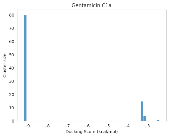
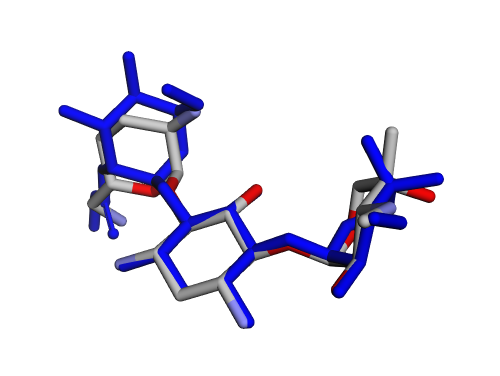
From the docking results above, we can conclude that a highly energetically favoured conformation for Gentamicin C1a exists. However, we cannot directly assume whether the method is efficient in reproducing the crystallographic pose yet. While visual inspection provides a qualitative idea, a more rigorous and quantitative metric is the Root Mean Square Deviation (RMSD), which measures the average distance between equivalent atoms in two structures. In this context, we will calculate the RMSD between each of the four docked poses identified by AutoDock and the crystallographic reference ligand. This allows us to objectively assess how closely the docking protocol is able to replicate the experimentally observed binding mode.
Calculate RMSD
#In a python terminal, run the following code:
  import os, glob
  import numpy as np
  from rdkit import Chem
  from rdkit.Chem import AllChem
  import pandas as pd

  def rmsd_ref_vs_pdb_glob(ref_pdb: str, pdb_glob: str, *, remove_hs: bool = False, sanitize: bool = True, sort_by: str = "RMSD", save_csv: str | None = None,
  ) -> pd.DataFrame:
      ref = Chem.MolFromPDBFile(ref_pdb, sanitize=sanitize, removeHs=False)
      if ref is None and sanitize:
          ref = Chem.MolFromPDBFile(ref_pdb, sanitize=False, removeHs=False)
      if ref is None:
          raise ValueError(f"Failed reference PDB: {ref_pdb}")

      ref_mol = Chem.RemoveHs(ref) if remove_hs else ref
      n_ref = ref_mol.GetNumAtoms()

      results = []
      files = sorted(glob.glob(pdb_glob))
      if not files:
          raise FileNotFoundError(f"PDB files matching {pdb_glob} not found")

      for pdb_file in files:
          pose_name = os.path.splitext(os.path.basename(pdb_file))[0]
          notes = ""
          rmsd_val = np.nan

          try:
              mol = Chem.MolFromPDBFile(pdb_file, sanitize=sanitize, removeHs=False)
              if mol is None and sanitize:
                  mol = Chem.MolFromPDBFile(pdb_file, sanitize=False, removeHs=False)
              if mol is None:
                  notes = "MolFromPDBFile = None"
              else:
                  mol_m = Chem.RemoveHs(mol) if remove_hs else mol
                  n_pose = mol_m.GetNumAtoms()

                  if n_pose != n_ref:
                      notes = f"Atoms do not match (ref={n_ref}, pose={n_pose})"
                  else:
                      rmsd_val = AllChem.GetBestRMS(ref_mol, mol_m)
          except Exception as e:
              notes = f"ERROR: {e}"
              n_pose = np.nan

          results.append({
              "Pose": pose_name,
              "RMSD": rmsd_val,
          })

      df = pd.DataFrame(results)
      if sort_by in df.columns:
          df = df.sort_values(sort_by, na_position="last").reset_index(drop=True)
      else:
          df = df.sort_values("Pose").reset_index(drop=True)

      if save_csv:
          df.to_csv(save_csv, index=False)

      return df

  #Please check the paths and adapt them to your own system.
  df = rmsd_ref_vs_pdb_glob(
      ref_pdb="/Aminoglycosides/docking/raw_data/genta_target/genta.pdb",
      pdb_glob="/Aminoglycosides/docking/docking_assays/assay_1/docked_1_per_cluster/VEGXETMJINRLTH-*.pdb",
      sort_by="RMSD",
      save_csv="rmsd_GentamicinC1a.csv"
  )
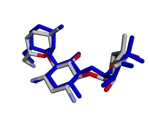
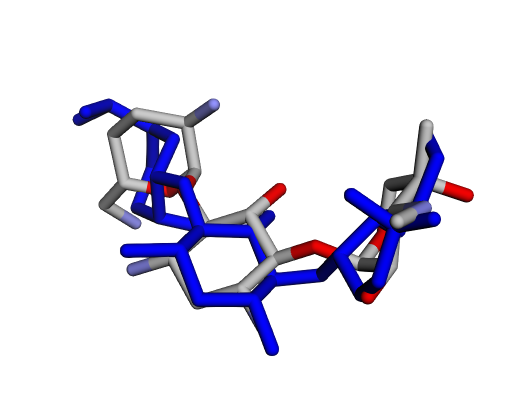
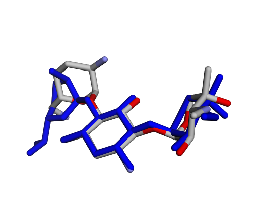
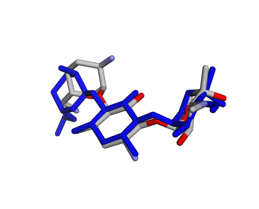
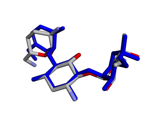
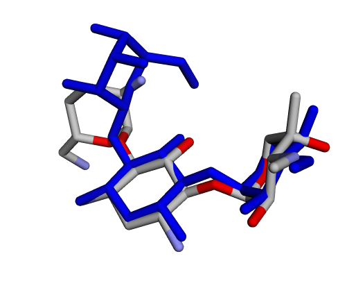
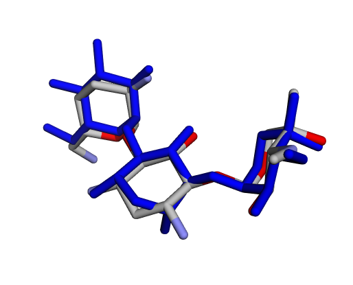
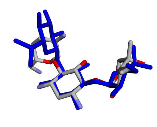
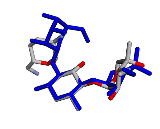
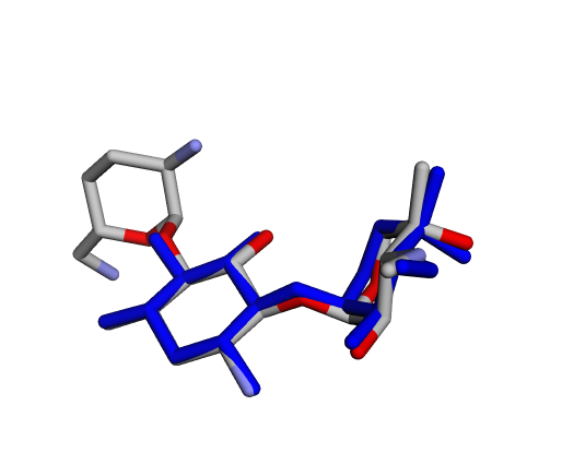
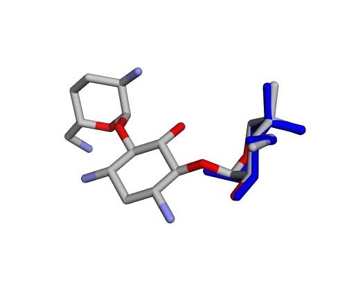
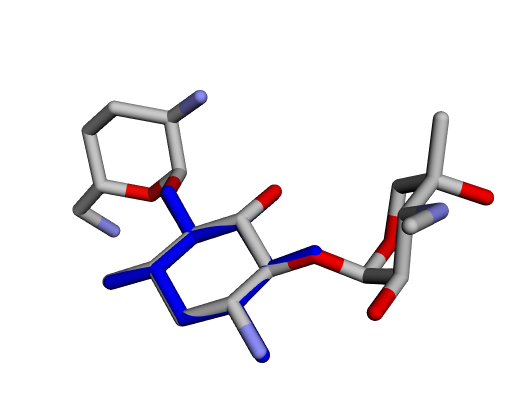
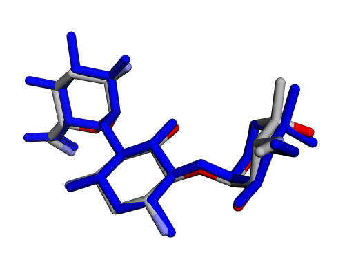
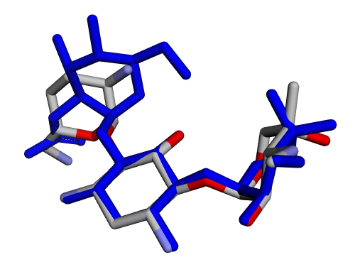
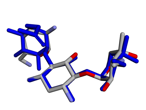
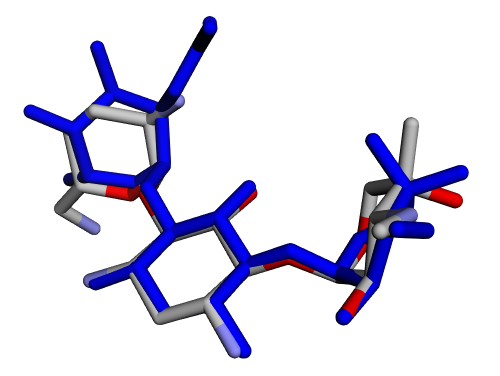
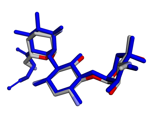
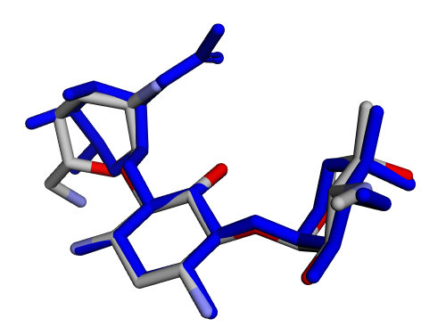
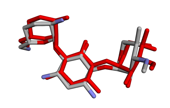 (a) Crystallographic GentamicinC1a vs Docked Pose 1 (red) (a) Crystallographic GentamicinC1a vs Docked Pose 1 (red) | 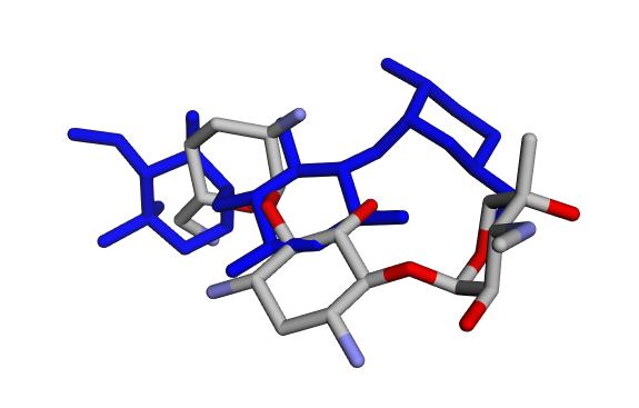 (b) Crystallographic GentamicinC1a vs Docked Pose 2 (blue) (b) Crystallographic GentamicinC1a vs Docked Pose 2 (blue) |
|---|---|
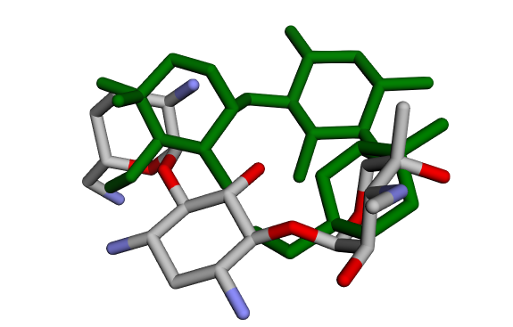 (c) Crystallographic GentamicinC1a vs Docked Pose 3 (green) (c) Crystallographic GentamicinC1a vs Docked Pose 3 (green) | 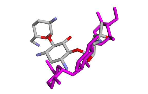 (d) Crystallographic GentamicinC1a vs Docked Pose 4 (pink) (d) Crystallographic GentamicinC1a vs Docked Pose 4 (pink) |
| Pose | RMSD |
|---|---|
| GentamicinC1a_1 | 0.277755 |
| GentamicinC1a_2 | 2.958624 |
| GentamicinC1a_3 | 2.248772 |
| GentamicinC1a_4 | 2.947599 |
Taken together, the visual overlays and the RMSD calculations consistently indicate that only the first docked pose (GentamicinC1a_1, Fig 11a) reproduces the crystallographic binding mode with high accuracy (RMSD < 0.3 Å). In contrast, the other poses display large deviations (> 2 Å), confirming that they represent alternative orientations rather than the native binding conformation. This combined qualitative and quantitative evaluation validates the docking setup.
1.5.2. Computing interaction fingerprints for a docked pose
The function compute_fingerprints_for_docked_pose() automates the post-processing of one specific docked pose, generating:
- per-residue ProLIF interaction fingerprints (binary interaction features),
- per-residue MMGBSA interaction fingerprints (AMBER MMPBSA decomposition).
aminoglycosides_example_docking_analysis.compute_fingerprints_for_docked_pose(
    assay_id,
    results_pose_id,
    mmgbsa=1,
    prolif=1,
    clean_files=1,
    clean_folder=1,
    solvent="implicit",
    min_steps=5000,
    store_docked_poses=1,
    prolif_parameters_set=1,
    iteration=1,
    ligresname="UNL",
)
Parameters
-
assay_id (int, required): ID of the docking assay containing the pose.
-
results_pose_id (int, required): ID of the pose to analyze (from the assay database results, e.g.: assay_X.pdb).
-
mmgbsa (0/1, default=1): compute (1) or not (0) MMGBSA per-residue decomposition for the pose.
-
prolif (0/1, default=1): compute (1) or not (0) ProLIF interaction fingerprint for the pose.
-
clean_files (0/1, default=1): remove (1) or not (0) temporary files generated by MMPBSA/LEaP after finishing.
-
clean_folder (0/1, default=1): remove (1) or not (0) the whole fingerprints_analyses/working folder after storing outputs.
-
solvent (explicit, default="implicit"): solvent model used during minimization/prep for fingerprints.
-
min_steps (int, default=5000): minimization steps for preparing the complex prior to fingerprints.
-
store_docked_poses (0/1, default=1): store (1) or not (0) the docked pose in the results DB.
-
prolif_parameters_set (int, default=1): ID of the parameter set in docking/params/prolif_parameters.db.
-
iteration (int, default=1): if 1, builds a residue-mapping dictionary (crystal vs tleap) and saves it; otherwise reuses it.
-
ligresname (str, default="UNL"): residue name used for the ligand in the complex (needed by LEaP/MMPBSA).
🤔 What does the function do?
i) Sets up a working directory under docking/docking_assays/assay_<ID>/fingerprints_analyses/<pose_subfolder>/.
ii) If mmgbsa == 1, prepares AMBER input (LEaP), minimizes the complex (min_steps, solvent), runs MMPBSA decomposition and writes a per-residue CSV, and stores the results in the DB (store_mmbgsa_fingerprints_results_in_db).
iii) If prolif == 1, builds a reference ProLIF dataframe for the entire receptor, mapped to the crystallographic numbering. It reuses the minimized prmtop/crd files if mmgbsa == 1; otherwise, these files are generated specifically for the ProLIF computation. Then, it retrieves the parameter set from docking/params/prolif_parameters.db according to the prolif_parameters_set ID, computes the ProLIF fingerprint for the docked pose and maps it to the crystallographic residue numbering, and saves the results as prolif_fingerprints_renum.csv and registers them in the database.
iv) If store_docked_poses == 1, the pose itself is stored in the results database.
v) Depending on the values of clean_files and clean_folder, the function will also remove intermediate files and/or the entire workspace once the computations are complete.
vi) Finally, the total execution time is logged and printed to the console.
As a practical example, we will calculate the interaction fingerprint of Gentamicin C1a docked pose 1, in order to evaluate whether the interactions identified experimentally can also be reproduced in silico. For simplicity, we will use the default conditions of the function.
aminoglycosides_example_docking_analysis.compute_fingerprints_for_docked_pose(assay_id=1, results_pose_id=1)
1.5.2.1. Interaction fingerprints with ProLIF
ProLIF is a Python library that encodes target–ligand interactions into machine-readable fingerprints.
For each residue, it records whether specific interaction types were detected with the ligand in a given pose.
What information does it provide?
Each column of the output corresponds to a residue–interaction pair, for example:
G2_A_HBDonor→ hydrogen bond donor detected between residue G2 of RNA chain A and the ligand.C3_A_PiStacking→ π–π stacking between residue C3 and the ligand.U5_A_CationPi→ cation–π interaction with residue U5.A7_A_VdWContact→ van der Waals contact between residue A7 and the ligand.
Values are binary (0 or 1), indicating the presence (1) or absence (0) of the interaction in a given pose.
This way, each pose can be represented as a vector of interactions, allowing systematic comparisons between poses or ligands.
How to analyze it?
- At the single-pose level, you can identify which key interactions (e.g., H-bonds, hydrophobic contacts) stabilize the binding mode.
- At the comparative level, you can check whether the best-scoring poses reproduce the same interactions observed in the crystallographic structure (e.g., conserved H-bonds in the A-site).
- At the dataset level, these fingerprints can be clustered or used as features in QSAR/ML models to link interaction patterns with biological activity.
To facilitate the interpretation of the raw ProLIF output, we reformatted the .csv file into a tidy table where each row corresponds to a residue–interaction pair. In a python terminal, run the following code:
import re
import pandas as pd

df = pd.read_csv('*docking/docking_assays/assay_1/fingerprints_analyses/pose_1/prolif_fingerprints_renum.csv*')

row = df.iloc[0]
records = []
pat = re.compile(r'^(?P<res>[ACGUT]\d+_[A-Z])_(?P<int>.+)$')  # ajustá si usás otra nomenclatura
for col, val in row.items():
    m = pat.match(col)
    if m:
        records.append((m.group("res"), m.group("int"), int(val)))

tidy = pd.DataFrame(records, columns=["Residue", "Interaction", "Value"])
print(tidy)
| index | Residue | Interaction | Value |
|---|---|---|---|
| 35 | G4_A | HBAcceptor | 1 |
| 36 | G4_A | HBDonor | 1 |
| 37 | G4_A | Hydrophobic | 1 |
| 42 | G4_A | VdWContact | 1 |
| 50 | U5_A | HBAcceptor | 1 |
| 57 | U5_A | VdWContact | 1 |
| 77 | A7_A | Cationic | 1 |
| 80 | A7_A | HBAcceptor | 1 |
| 81 | A7_A | HBDonor | 1 |
| 82 | A7_A | Hydrophobic | 1 |
| 87 | A7_A | VdWContact | 1 |
| 542 | A40_B | Cationic | 1 |
| 545 | A40_B | HBAcceptor | 1 |
| 546 | A40_B | HBDonor | 1 |
| 547 | A40_B | Hydrophobic | 1 |
| 552 | A40_B | VdWContact | 1 |
| 557 | G41_B | Cationic | 1 |
| 560 | G41_B | HBAcceptor | 1 |
| 561 | G41_B | HBDonor | 1 |
| 567 | G41_B | VdWContact | 1 |
| 572 | U42_B | Cationic | 1 |
| 575 | U42_B | HBAcceptor | 1 |
| 576 | U42_B | HBDonor | 1 |
| 577 | U42_B | Hydrophobic | 1 |
| 582 | U42_B | VdWContact | 1 |
| 0 | G2_A | Anionic | 0 |
| 1 | G2_A | CationPi | 0 |
| 2 | G2_A | Cationic | 0 |
| 3 | G2_A | EdgeToFace | 0 |
| 4 | G2_A | FaceToFace | 0 |
| 5 | G2_A | HBAcceptor | 0 |
| ... | ... | ... | ... |
The resulting table shows that several residues contribute multiple contacts, including G4A, U5A, A7A, A40B, G41B, and U42B, each displaying a combination of hydrogen bonds, hydrophobic/van der Waals contacts, and cationic interactions. In contrast, many other residues remain inactive (all values = 0), indicating that only a subset of the RNA helix may be directly involved in ligand recognition.
To provide an overview at the residue level, we can visually compare the reported and in silico fingerprints.
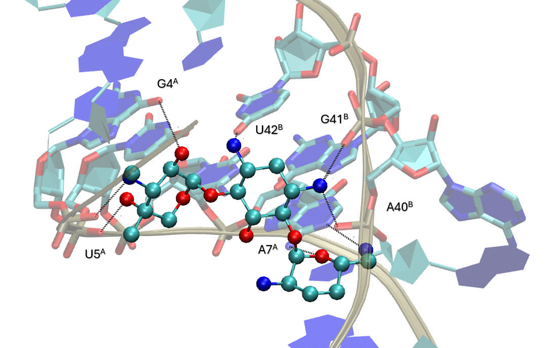
Together, those outputs confirm that the docking-derived fingerprint captures the main contacts observed experimentally. This strengthens the confidence in the docking protocol and illustrates the utility of ProLIF fingerprints for a residue-level analysis of docking results.
1.5.2.2. Interaction fingerprints with MMGBSA
In addition to ProLIF, TidyScreen provides the option to minimize the docked pose of interest and evaluate the energetic contribution of each residue to the complex stabilization through MMGBSA per-residue decomposition. This approach not only reveals which contacts are present, but also quantifies how favorable or unfavorable each interaction is. Furthermore, it allows the calculation of the overall Effective Binding Energy (EBE) of the complex.
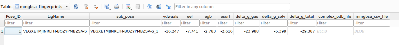
By setting mmgbsa = 1 in the compute_fingerprints_for_docked_pose() function, a file named mmgbsa_DECOMP_renum.csv is generated, and a new mmgbsa_fingerprints table is added to the assay_<ID>.db database.
Interestingly, analysis of Gentamicin C1a highlights a marked difference between the MMGBSA-derived EBE (-29.4 kcal/mol) and the AutoDock docking score (-9.2 kcal/mol). While docking scores are useful for ranking poses, MMGBSA provides a more physically grounded estimation of binding affinity, often better correlated with experimental data. This illustrates the added value of complementing docking with energetic refinement.
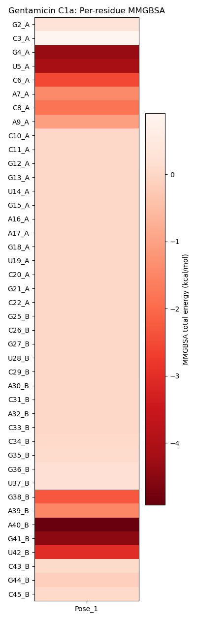
To facilitate interpretation, the .csv file can be visualized as a heatmap, where each residue is represented by its total energy contribution.
Run the following code in a Python terminal:
import pandas as pd
import matplotlib.pyplot as plt
df = pd.read_csv("*/docking/docking_assays/assay_1/fingerprints_analyses/pose_1/mmgbsa_DECOMP_renum.csv")

df["Residue"] = df["resname"] + df["resnumber"].astype(str) + "_" + df["chain"]
df = df.sort_values("resnumber")
matrix = df[["total"]].copy()
matrix.index = df["Residue"]
matrix.columns = ["Pose_1"]
plt.figure(figsize=(4, len(df)*0.3))
im = plt.imshow(matrix, cmap="Reds_r", aspect="auto")
cbar = plt.colorbar(im)
cbar.set_label("MMGBSA total energy (kcal/mol)")
plt.yticks(range(len(df)), df["Residue"])
plt.xticks([0], ["Pose_1"])
plt.title("Per-residue MMGBSA decomposition")
plt.tight_layout()
plt.show()
plt.savefig("GentamicinC1a_mmgbsa_DECOMP.png")
The resulting heatmap shows that the main residues identified in docking (G4, U5, A7, A40, G41, and U42) also appear as the most stabilizing according to MMGBSA. In addition, new contributors such as C6, C8, A9, G38, and A39 emerge, reflecting subtle rearrangements in orientations and distances after minimization. These findings highlight the complementarity between contact-based (ProLIF) and energy-based (MMGBSA) fingerprints.
1.6. Conclusion
By systematically replicating the crystallographic binding mode of Gentamicin C1a, we validated the reliability of the docking protocol implemented in TidyScreen.
Visual inspection and RMSD analysis confirmed that the top-ranked pose reproduces the experimental conformation with sub-angstrom accuracy, while alternative poses correspond to less relevant orientations.
Interaction fingerprints provided complementary evidence:
- ProLIF captured the network of contacts in line with the crystallographic observations (i.e., G4, U5, A7, A40, G41, U42).
- MMGBSA not only reinforced the role of these key residues but also revealed additional contributors (i.e., C6, C8, A9, G38, A39) that stabilize the minimized complex.
Together, these results demonstrate that combining docking with quantitative metrics (RMSD), contact-based fingerprints (ProLIF), and energetic decomposition (MMGBSA) offers a robust framework for assessing docking performance. This integrated approach not only validates the procedure against experimental data but also provides deeper insights into the molecular determinants of binding that can guide future virtual screening and drug design efforts.
2. Major and minor components of Gentamicin: pharmacodynamic insights into potency
Having validated our docking workflow by successfully reproducing the crystallographic pose of Gentamicin C1a, we now extend the analysis to the full spectrum of Gentamicin components.
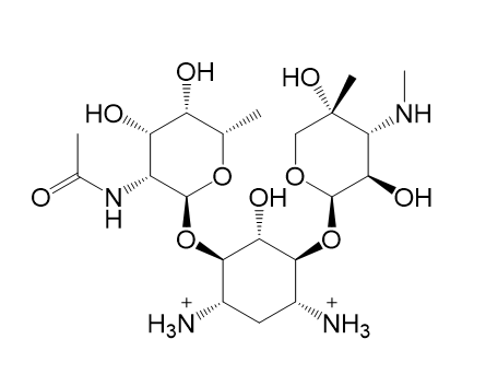
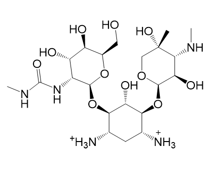
Commercial Gentamicin is supplied as a mixture of structurally related congeners. Among them, C1, C1a, C2, C2a, C2b, and sisomicin are reported to retain strong antibacterial potency when tested individually, while other components such as Gentamicin A, B, B1, X2, garamine, 2-deoxystreptamine, and garosamine display significantly weaker activity.
In this section, we aim to explore whether these differences in experimental potency may be explained, at least in part, by distinct interaction profiles with the ribosomal target.
At the same time, this analysis provides an additional layer of validation for our docking protocol: if the most favourable predicted poses for each congener align with the experimentally observed reference pose, it reinforces the robustness of the approach.
To achieve this, we will replicate the steps previously outlined:
- Import and parametrize each Gentamicin component from their SMILES.
- Perform docking studies.
- Analyse docked poses and evaluate interaction fingerprints using ProLIF.
- Complement the analysis with MMGBSA per-residue decomposition.
2.1. Gentamicin components
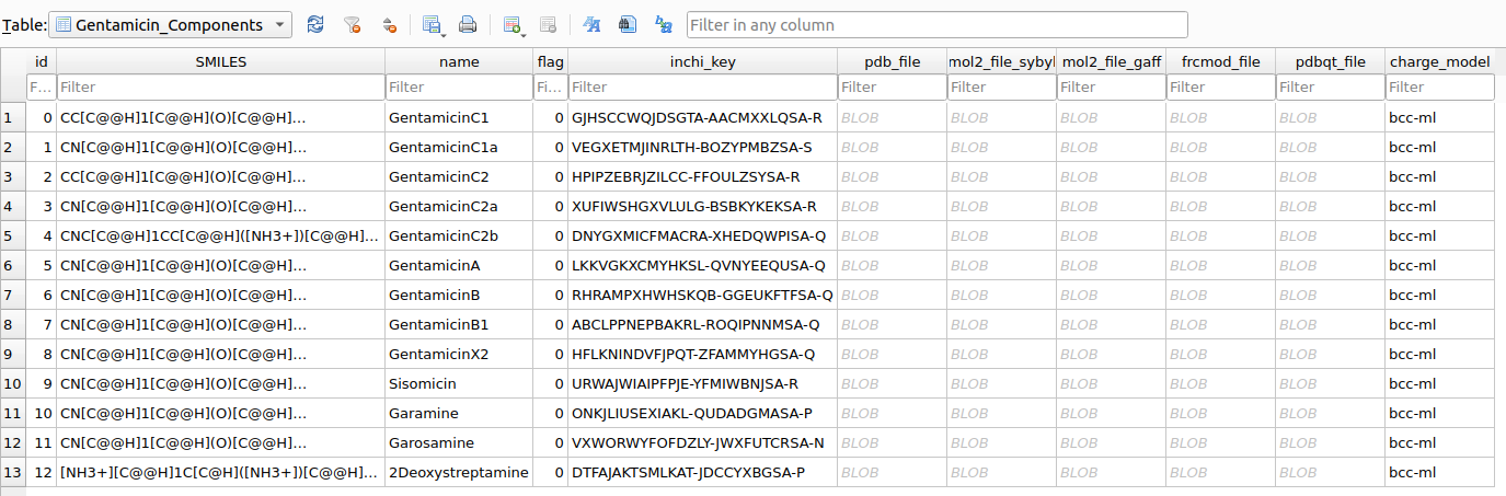
First, create a file called Gentamicin_Components.csv containing the SMILES of the ligands in the $HOME/Desktop/example/Aminoglycosides/chemspace/raw_data/ folder.
CC[C@@H]3[C@@H](O)[C@@H](O[C@H]2[C@H]([NH3+])C[C@H]([NH3+])[C@@H](O[C@H]1O[C@H]([C@@H](C)[NH2+]C)CC[C@H]1[NH3+])[C@@H]2O)OC[C@]3(C)O,GentamicinC1
CN[C@@H]3[C@@H](O)[C@@H](O[C@H]2[C@H]([NH3+])C[C@H]([NH3+])[C@@H](O[C@H]1O[C@H](C[NH3+])CC[C@H]1[NH3+])[C@@H]2O)OC[C@]3(C)O,GentamicinC1a
CC[C@@H]3[C@@H](O)[C@@H](O[C@H]2[C@H]([NH3+])C[C@H]([NH3+])[C@@H](O[C@H]1O[C@H]([C@@H](C)[NH3+])CC[C@H]1[NH3+])[C@@H]2O)OC[C@]3(C)O,GentamicinC2
CN[C@@H]3[C@@H](O)[C@@H](O[C@H]2[C@H]([NH3+])C[C@H]([NH3+])[C@@H](O[C@H]1O[C@H]([C@H](C)[NH3+])CC[C@H]1[NH3+])[C@@H]2O)OC[C@]3(C)O,GentamicinC2a
CNC[C@@H]3CC[C@@H]([NH3+])[C@@H](O[C@@H]2[C@@H]([NH3+])C[C@@H]([NH3+])[C@H](O[C@H]1OC[C@](C)(O)[C@H](NC)[C@H]1O)[C@H]2O)O3,GentamicinC2b
CN[C@H]3[C@H](O)CO[C@H](O[C@H]2[C@H]([NH3+])C[C@H]([NH3+])[C@@H](O[C@H]1O[C@H](CO)[C@@H](O)[C@H](O)[C@H]1[NH3+])[C@@H]2O)[C@@H]3O,GentamicinA
CN[C@@H]3[C@@H](O)[C@@H](O[C@H]2[C@H]([NH3+])C[C@H]([NH3+])[C@@H](O[C@H]1O[C@H](C[NH3+])[C@@H](O)[C@H](O)[C@H]1O)[C@@H]2O)OC[C@]3(C)O,GentamicinB
CN[C@@H]3[C@@H](O)[C@@H](O[C@H]2[C@H]([NH3+])C[C@H]([NH3+])[C@@H](O[C@@H]1O[C@H]([C@@H](C)[NH3+])[C@@H](O)[C@H](O)[C@H]1O)[C@@H]2O)OC[C@]3(C)O,GentamicinB1
CN[C@@H]3[C@@H](O)[C@@H](O[C@H]2[C@H]([NH3+])C[C@H]([NH3+])[C@@H](O[C@H]1O[C@H](CO)[C@@H](O)[C@H](O)[C@H]1[NH3+])[C@@H]2O)OC[C@]3(C)O,GentamicinX2
CN[C@@H]3[C@@H](O)[C@@H](O[C@H]2[C@H]([NH3+])C[C@H]([NH3+])[C@@H](O[C@H]1OC(C[NH3+])=CC[C@H]1[NH3+])[C@@H]2O)OC[C@]3(C)O,Sisomicin
CN[C@@H]2[C@@H](O)[C@@H](O[C@H]1[C@H]([NH3+])C[C@H]([NH3+])[C@@H](O)[C@@H]1O)OC[C@]2(C)O,Garamine
C[C@@]1(CO[C@@H]([C@@H]([C@H]1NC)O)O)O,Garosamine
[NH3+][C@@H]1C[C@H]([NH3+])[C@@H](O)[C@H](O)[C@H]1O,2Deoxystreptamine
Next, reactivate the ChemSpace module in Aminoglycosides.py, import the file, and generate the corresponding molecular files (.pdb, .pdbqt, .mol2, .frcmod).
aminoglycosides_example_chemspace = chemspace.ChemSpace(Aminoglycosides_example)
aminoglycosides_example_chemspace.input_csv("$HOME/Desktop/example/Aminoglycosides/chemspace/raw_data/Gentamicin_Components.csv")
aminoglycosides_example_chemspace.generate_mols_in_table("Gentamicin_Components", timeout=10000)
As a result, a Gentamicin_Components table will be created within the chemspace/processed_data/chemspace.db database.
.pdb, .pdbqt, .mol2, and .frcmod) after parameterization. At this point, all the necessary input files have been successfully prepared, and we are ready to proceed with the docking studies.
To proceed, we first activate the moldock module from TidyScreen and register the prepared receptor by creating a database entry that points to the target files (.map grids, .pdbqt, .fld, and reference .pdb).
2.2. Molecular Docking
Now, we will run the docking study for the complete set of Gentamicin components, using the same conditions defined in Section 1. This will allow us to compare the binding profiles of all major and minor congeners under identical parameters.
# Initialize MolDock
aminoglycosides_example_docking = moldock.MolDock(Aminoglycosides_example)
# Run docking for the full Gentamicin component set
aminoglycosides_example_docking.dock_table(table_name="Gentamicin_Components", id_receptor_model=1, id_docking_params=2)
After execution, a new assay will be registered in the docking/docking_registers.db, and a dedicated folder will be created inside docking/docking_assays/, containing all input/output files and the docking_execution.sh script ready to run the assay.
You can launch the assay in your terminal with:
./docking_execution.sh
When the docking study is complete, the results can be processed using the same workflow described before. This step will extract the docked poses, summarize docking scores, cluster sizes, and optionally generate .pdb files for visualization. By doing so, we can directly compare the binding profiles of all Gentamicin components under the same conditions.
#Set and run the docking analysis
aminoglycosides_example_docking_analysis.process_docking_assay(assay_id=2, max_poses=10, vmd_path="PATH/TO/VMD", extract_poses=1)
The analysis will generate an assay_<ID>.db file containing docking results for each ligand/pose, as well as a docked_1_per_cluster/ folder with the poses extracted for subsequent analyses.
Let's analyze the results. As a first step, since we re-docked Gentamicin C1a, it is important to check if the outcome was consistent with our previous run in Section 1.5. Indeed, the results were highly comparable: the top-ranked pose showed a docking score of -9.25 kcal/mol, a cluster size of 80, and an RMSD of 0.281 Å with respect to the crystallographic pose. This highlights the reproducibility of the method and validates the robustness of the setup.
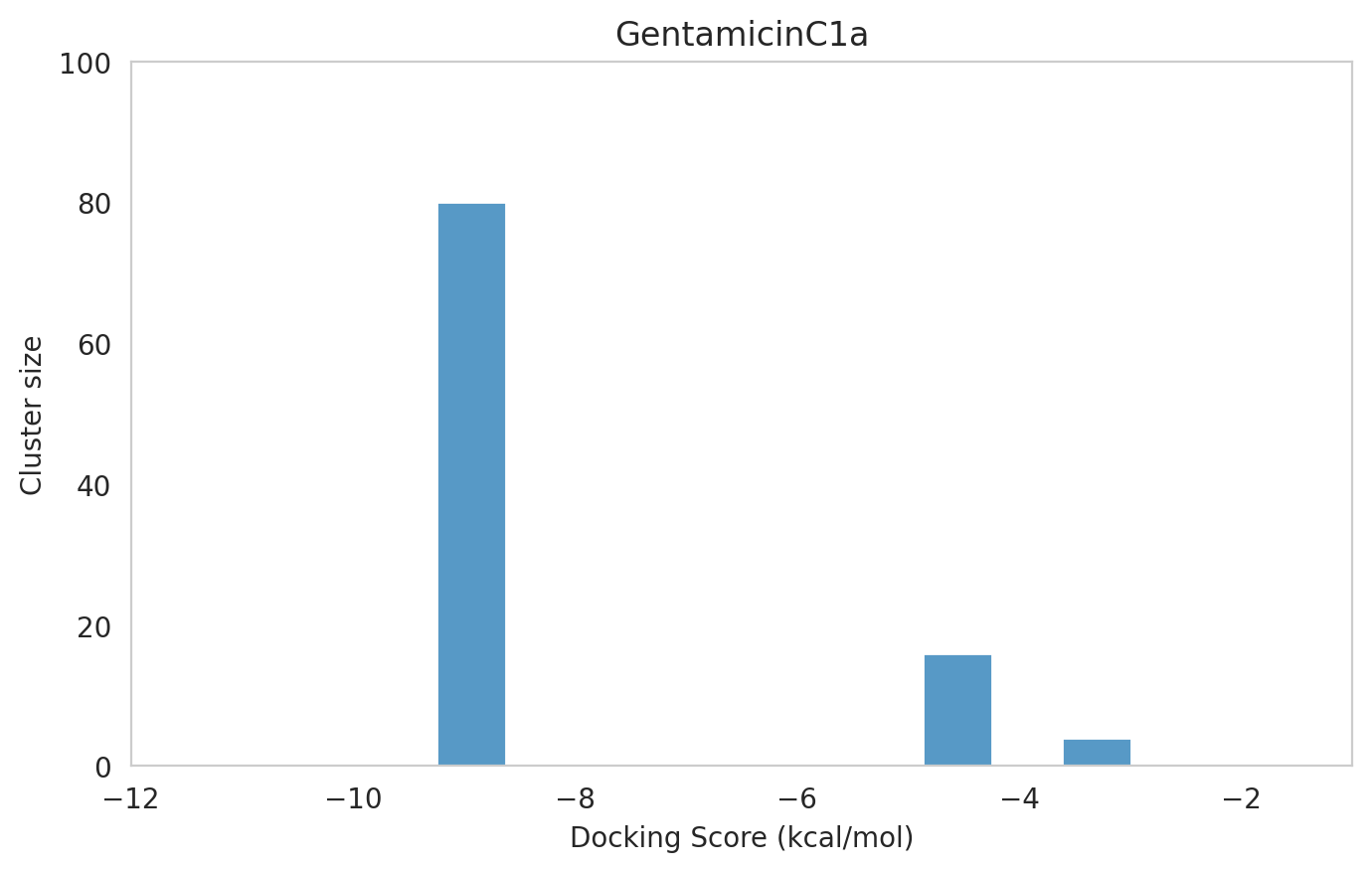
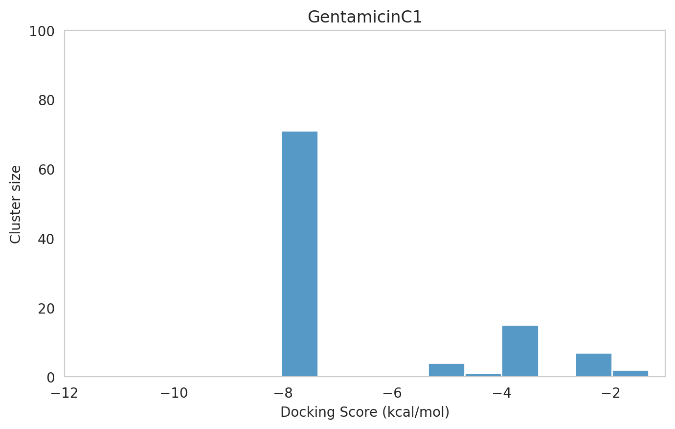
We next examined the docking histograms for all Gentamicin components to identify potential trends.
 | 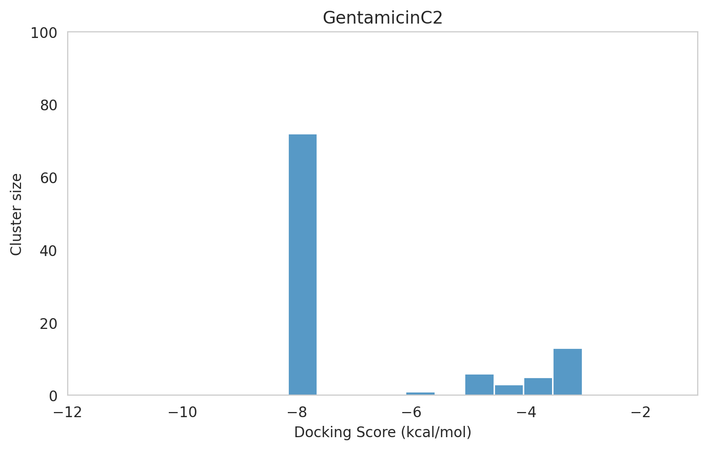 | 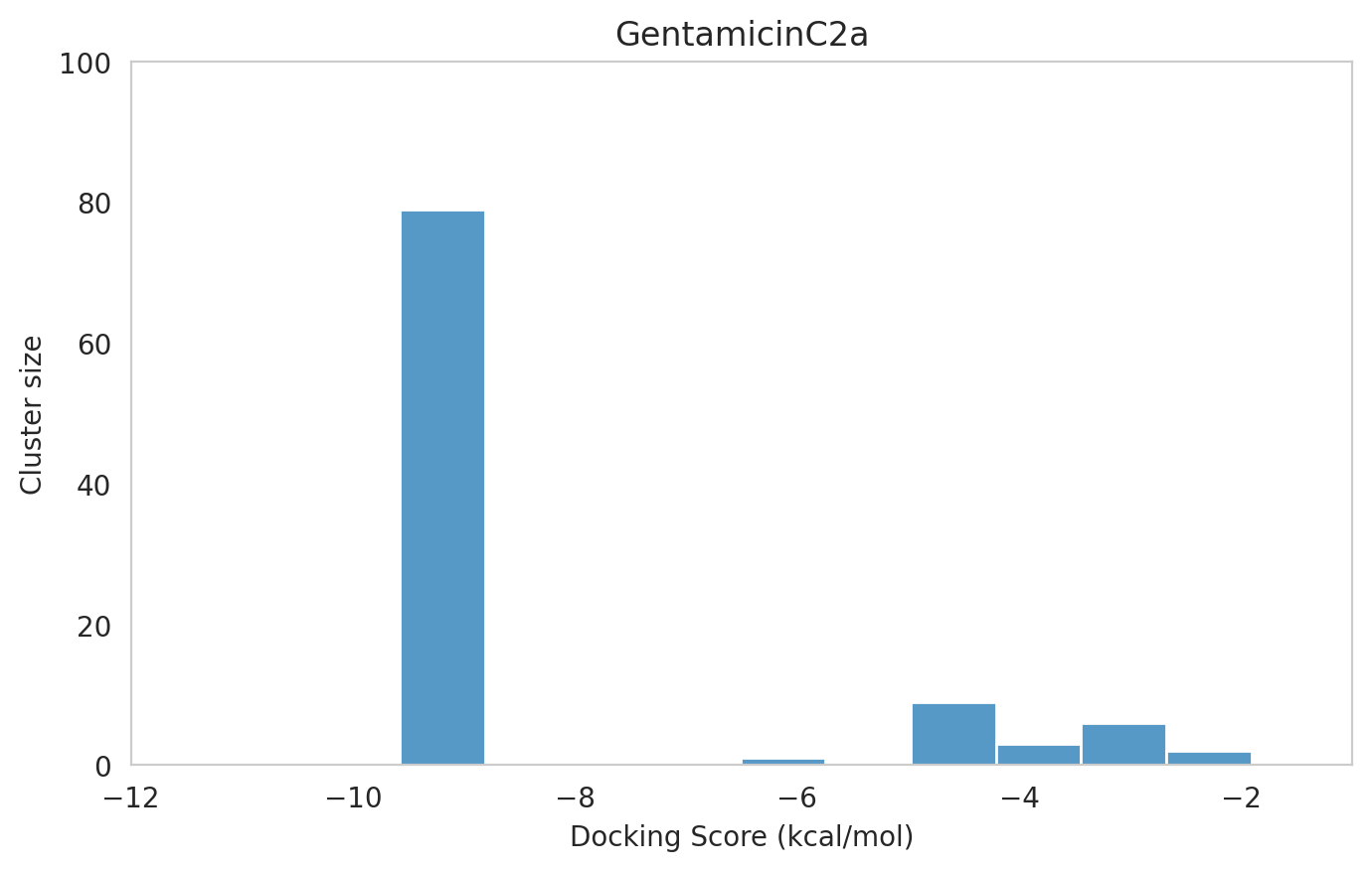 |
|---|---|---|
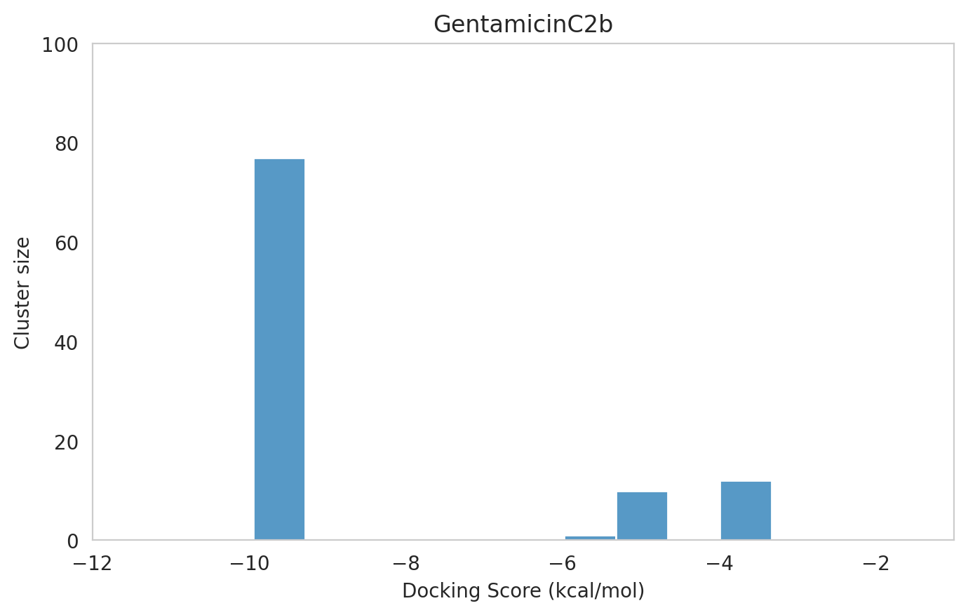 | 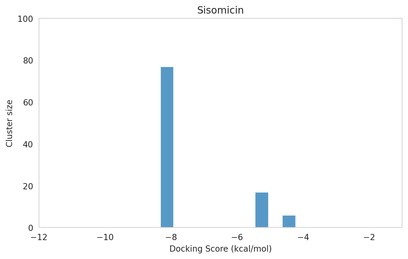 | 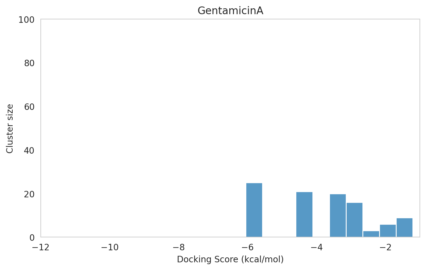 |
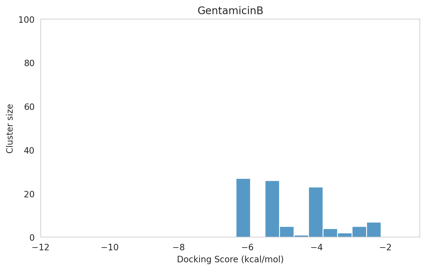 | 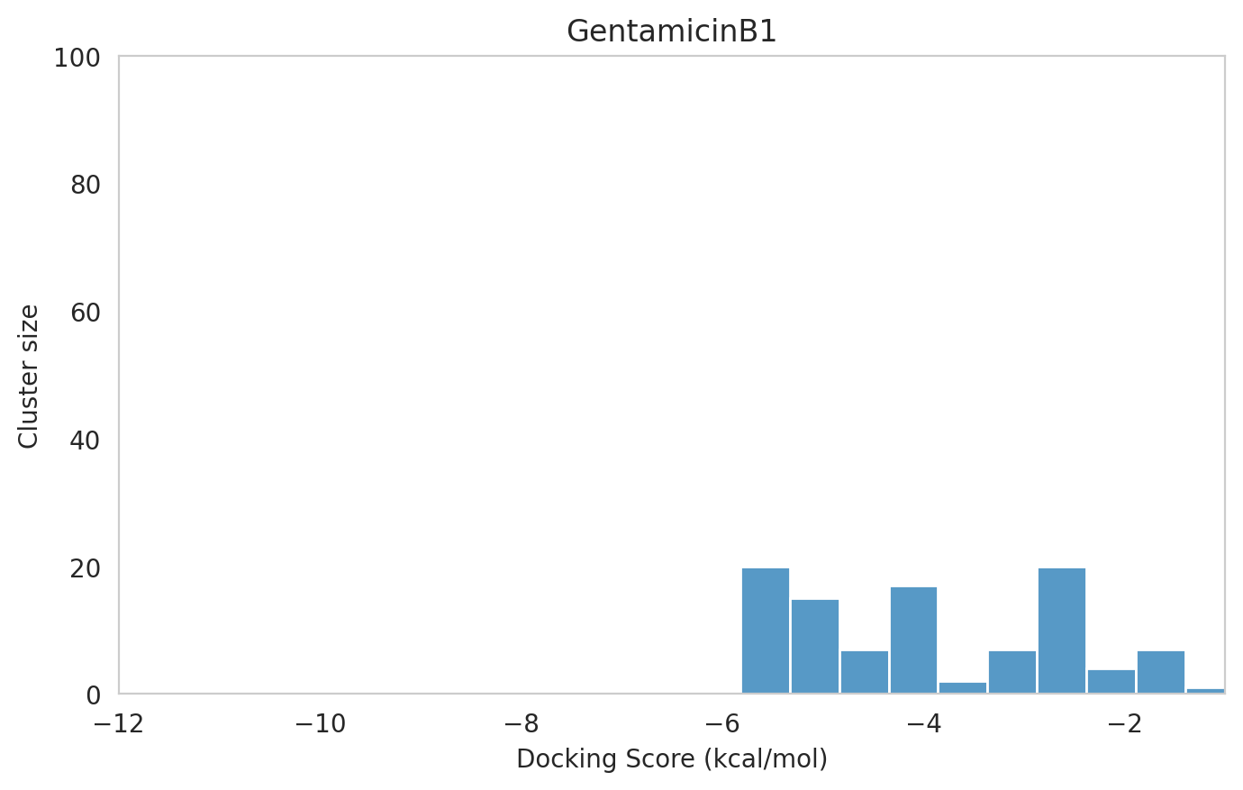 | 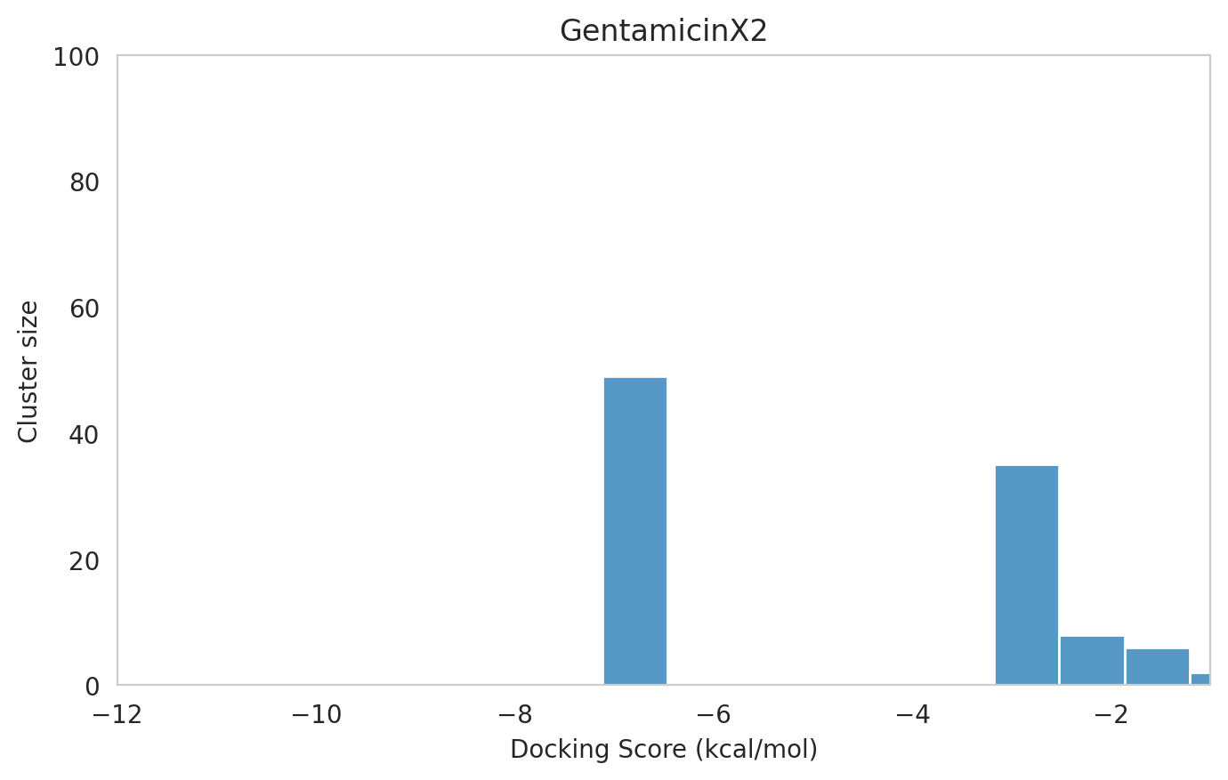 |
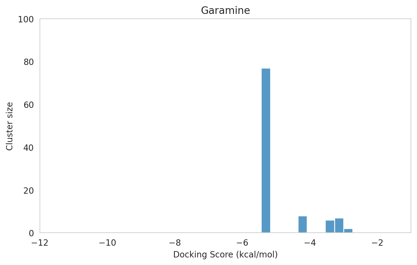 | 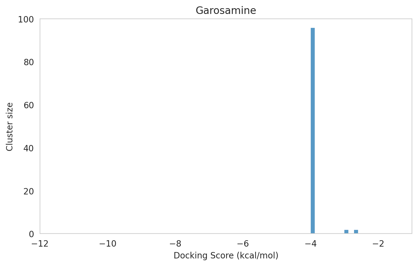 | 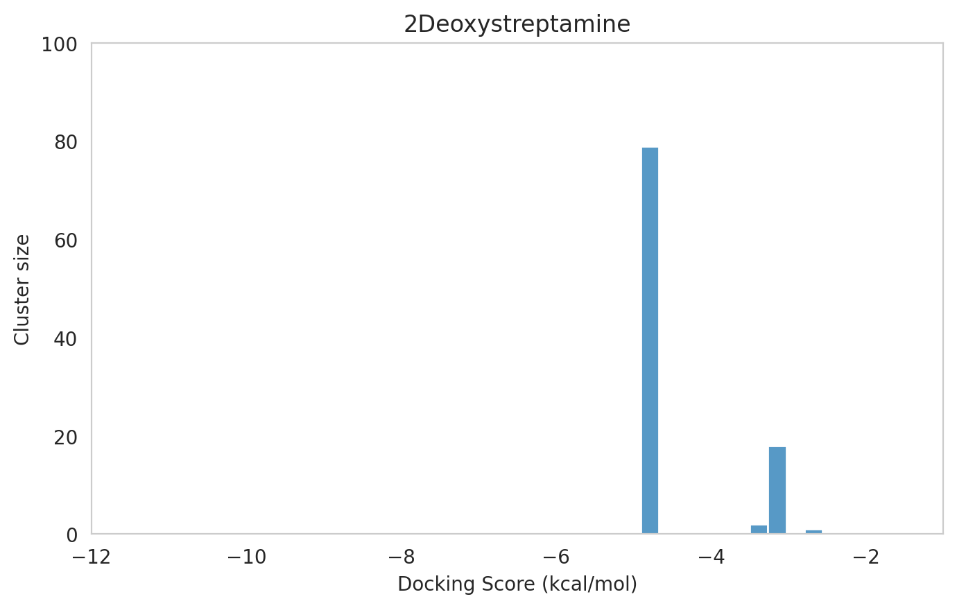 |
The most potent components (Gentamicins C and Sisomicin) consistently showed a well-defined, energetically favoured pose, with docking scores between -10 and -7 kcal/mol and cluster sizes of 70-80. In contrast, the minor components (i.e. Gentamicin X2, A, B, and B1; Garamine, Garosamine, and 2-Deoxystreptamine) yielded higher scores (-6.5 to -4 kcal/mol) and more heterogeneous conformer distributions, with cluster sizes between 20–43 for their best poses.
Interestingly, the smallest scaffolds (garamine, garosamine, 2-deoxystreptamine) displayed very high cluster sizes (77-96). A plausible explanation is their reduced conformational flexibility, which limits exploration of alternative binding modes and yields families of closely related poses that cluster together. In this dataset, those compounds did not show favorable docking scores, underscoring why both score and cluster size should be considered jointly: interpreting either metric in isolation can be misleading.
| index | Rank | Docking_score | Mean_score | Cluster_size | Ligand | Pose |
|---|---|---|---|---|---|---|
| 95 | 1 | -9.95 | -8.24 | 77 | GentamicinC2b | GentamicinC2b_1.pdb |
| 87 | 1 | -9.58 | -9.3 | 79 | GentamicinC2a | GentamicinC2a_1.pdb |
| 74 | 1 | -9.25 | -7.8 | 80 | GentamicinC1a | GentamicinC1a_1.pdb |
| 120 | 1 | -8.33 | -7.25 | 77 | Sisomicin | Sisomicin_1.pdb |
| 78 | 1 | -8.16 | -7.43 | 72 | GentamicinC2 | GentamicinC2_1.pdb |
| 64 | 1 | -8.03 | -6.93 | 71 | GentamicinC1 | GentamicinC1_1.pdb |
| 103 | 1 | -7.12 | -6.44 | 43 | GentamicinX2 | GentamicinX2_1.pdb |
| 28 | 1 | -6.34 | -5.11 | 27 | GentamicinB | GentamicinB_1.pdb |
| 13 | 1 | -6.05 | -5.68 | 25 | GentamicinA | GentamicinA_1.pdb |
| 39 | 1 | -5.82 | -5.09 | 20 | GentamicinB1 | GentamicinB1_1.pdb |
| 4 | 1 | -5.44 | -4.81 | 77 | Garamine | Garamine_1.pdb |
| 0 | 1 | -4.91 | -3.86 | 79 | 2Deoxystreptamine | 2Deoxystreptamine_1.pdb |
| 10 | 1 | -4.01 | -3.87 | 96 | Garosamine | Garosamine_1.pdb |
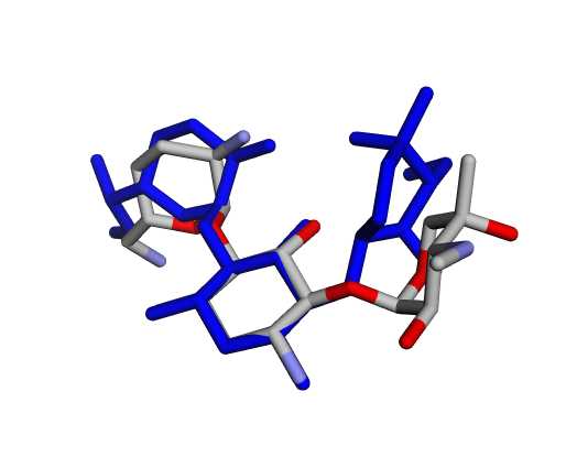 |  |  |
|---|---|---|
| (a) Gentamicin C1 | (b) Gentamicin C1a | (c) Gentamicin C2 |
 |  |  |
| (d) Gentamicin C2a | (e) Gentamicin C2b | (f) Sisomicin |
 |  |  |
| (g) Gentamicin A | (h) Gentamicin B | (i) Gentamicin B1 |
 |  |  |
| (j) Gentamicin X2 | (k) Garamine | (l) Garosamine |
 | ||
| (m) 2-Deoxystreptamine |
By confirming that the most populated and energetically favoured poses of the active components align with the crystallographic reference, we further validate the docking protocol. Moreover, these comparative analyses provide the first pharmacodynamic clues to explain the differential bioactivity of Gentamicin components.
To extend the analysis beyond a single ligand, TidyScreen provides the compute_fingerprints_for_whole_assay() function, which automates the post-processing of all docked ligands within a given assay, running both ProLIF and MMGBSA calculations in batch mode. In practice, the function works almost identically to compute_fingerprints_for_docked_pose() (Section 1.5.2.), but instead of specifying a single pose ID, the user only needs to indicate the assay_id.
aminoglycosides_example_docking_analysis.compute_fingerprints_for_whole_assay(assay_id=2)
Considering the ProLIF-derived fingerprints, a clear separation emerges between ligands that establish contacts with residue A7—which correspond to the most potent components—and those that do not, typically the least potent ones. As anticipated, the smaller scaffolds Garosamine and 2-Deoxystreptamine also lack additional stabilizing interactions across the pocket. Together, these trends point to A7 as a key nucleotide for potency within the ribosomal A-site.

While docking and ProLIF fingerprints provided valuable information on binding modes and contact patterns, the per-residue MMGBSA decomposition offers a complementary energetic perspective.
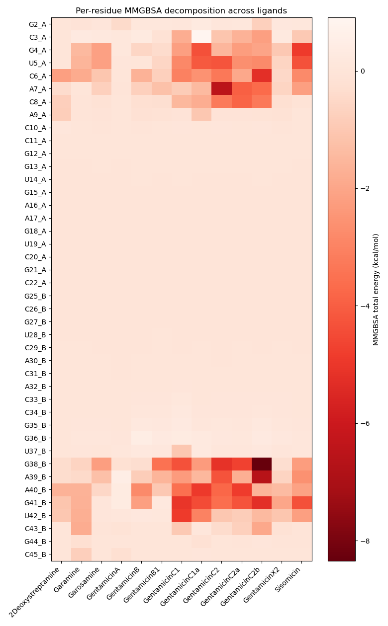
For Gentamicins C and Sisomicin, the analysis confirmed that residues already highlighted in docking (G4, U5, A7, A40, G41, U42) are also the most stabilizing, with additional contributors (C6, C8, A9, G38, A39) emerging after minimization. Extending this approach to the full panel of Gentamicin components revealed a consistent trend: minor or less potent components (X2, A, B, B1, Garamine, 2-Deoxystreptamine, Garosamine) show weaker stabilization, with diminished contributions and fewer cooperative contacts overall. This comparative analysis highlights how MMGBSA fingerprints complement docking-based metrics, by discriminating not only which residues are contacted but also which ones drive stabilization. In this way, MMGBSA strengthens the pharmacodynamic rationale behind the differential potency of Gentamicin components.
Altogether, these data validate a workflow that can now be leveraged for the massive screening of novel Gentamicin analogues, with the potential to deliver affordable compounds of enhanced antimicrobial activity.
2.3. Conclusion
Through a systematic docking, ProLIF, and MMGBSA analysis of all Gentamicin congeners, we were able to connect structural variation with pharmacodynamic consequences at the ribosomal A-site. The workflow not only reproduced the crystallographic pose of Gentamicin C1a with high accuracy, but also distinguished between major and minor components of the commercial mixture.
Active congeners (Gentamicins C1, C1a, C2, C2a, C2b, and Sisomicin) consistently engaged key nucleotides such as A7, G4, U5, A40, G41, and U42, establishing stabilizing contacts and favorable energetic profiles. In contrast, less potent species (Gentamicin A, B, B1, X2) and fragment-like scaffolds (Garamine, 2-Deoxystreptamine, Garosamine) lacked robust A7 engagement and displayed weaker energetic stabilization, providing a plausible molecular rationale for their diminished activity.
The integration of contact-based fingerprints (ProLIF) with energy-based fingerprints (MMGBSA) proved crucial: while ProLIF mapped the presence or absence of key pharmacophoric interactions, MMGBSA revealed which residues made the strongest stabilizing contributions after minimization. This complementary approach enabled a more nuanced discrimination between potent and weak components.
Overall, this section demonstrates that our validated workflow can recapitulate experimental potency trends within a heterogeneous mixture of natural products. This reinforces its reliability and sets the stage for prospecting novel Gentamicin analogues via virtual high-throughput screening, aimed at identifying affordable compounds with improved antimicrobial potential.
3. New Gentamicin analogues: vHTS
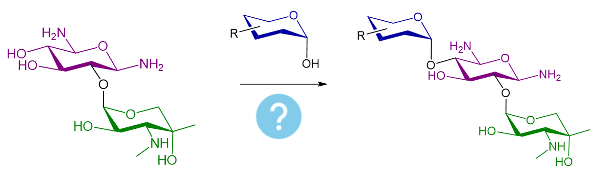
As shown above, the key pharmacodynamic differences across gentamicin derivatives largely trace back to structural variations on ring I. Here, we explore whether alternative ring I motifs can reproduce — or even improve — the interaction fingerprint of the most active components, nominating them as promising analogues.
To that end, we will in silico assemble a glycosidic bond between Garamine (common core) and diverse 2-tetrahydropyranol derivatives harvested from the eMolecules database, and then run a virtual high-throughput screening (vHTS) to compare outcomes side-by-side.
A dedicated tutorial covers ChemSpace in depth. Below we only show the minimal steps used here; if needed, refer to that tutorial for configuration details and advanced options.
# 1) Activate ChemSpace
aminoglycosides_example_chemspace = chemspace.ChemSpace(Aminoglycosides_example)

# 2) Import eMolecules (if not previously added)
aminoglycosides_example_chemspace.input_csv("$PATH/TO/emolecules.csv")

# 3) Inspect available SMARTS filters
aminoglycosides_example_chemspace.list_available_smarts_filters()

# 4) Add a SMARTS filter for 2-tetrahydropyranol
aminoglycosides_example_chemspace.add_smarts_filter("[#6]1[#6][#6]~[#6][OX2H0][CX4;H1]1[OX2H]","Tetrahydropyranol")

# 5) Confirm the new filter and note its ID
aminoglycosides_example_chemspace.list_available_smarts_filters()

# 6) Build a custom filtering workflow keeping one tetrahydropyranol and excluding isotopes (2H, 3H, 13C, 15N)
aminoglycosides_example_chemspace.create_smarts_filters_workflow({54:1, 6:0, 7:0, 8:0, 9:0})

# 7) Subset eMolecules with that workflow
aminoglycosides_example_chemspace.subset_table_by_smarts_workflow("emolecules", 1)

# 8) Compute basic properties
aminoglycosides_example_chemspace.compute_properties("emolecules_subset_1")

# 9) Apply a simple property filter to retain those with moderate size
aminoglycosides_example_chemspace.subset_table_by_properties("emolecules_subset_1",["MolWt<=250"])

# 10) Give the working subset a clearer name
aminoglycosides_example_chemspace.copy_table_to_new_name("emolecules_subset_1_subset_2","Tetrahydropyranol_for_Glycosylation")

# 11) Import Garamine as the common starting material. SMILES: CN[C@@H]2[C@@H](O)[C@@H](O[C@H]1[C@H]([NH3+])C[C@H]([NH3+])[C@@H](O)[C@@H]1O)OC[C@]2(C)O
aminoglycosides_example_chemspace.input_csv("$PATH/TO/Garamine.csv")

# 12) List available reaction workflows
aminoglycosides_example_chemspace.list_available_reactions_workflows()

# 13) Register a glycosylation reaction (generic SMARTS)
aminoglycosides_example_chemspace.add_smarts_reaction("[CX4H2:1][CX4:2]([#7:3])[CX4:4][OH:5].[OH:8][CX4:7][O:6]>>[CX4H2:1][CX4:2]([#7:3])[CX4:4][O:8][CX4:7][O:6]", "Glycosylation")

# 14) Confirm that the new reaction was added and note its ID
aminoglycosides_example_chemspace.list_available_reactions_workflows()

# 15) Add the reaction workflow to the project
aminoglycosides_example_chemspace.add_smarts_reaction_workflow([1])

# 16) Apply the reaction: pair Garamine with the THP subset
aminoglycosides_example_chemspace.apply_reaction_workflow(1, [["Garamine", "Tetrahydropyranol_for_Glycosylation"]])

# 17) Quick visual sanity-check of the products (random sample)
aminoglycosides_example_chemspace.depict_ligand_table("reaction_set_1", limit=25, random=True)
Overall, from an initial set of 18832 2-tetrahydropyranols extracted from eMolecules, we filtered down to 2526 candidates (MW ≤ 250 Da and without isotopes). By combining these with Garamine, we effectively in silico synthesized 2526 novel gentamicin derivatives featuring diverse Ring I modifications.
Now, we are ready to generate inputs, perform docking, and analyse the results.
# Parametrization
aminoglycosides_example_chemspace.generate_mols_in_table("reaction_set_1", timeout=10000)
# Initialize MolDock
aminoglycosides_example_docking = moldock.MolDock(Aminoglycosides_example)
# Run docking for the full Gentamicin component set
aminoglycosides_example_docking.dock_table(table_name="reaction_set_1", id_receptor_model=1, id_docking_params=2)
After execution, a new assay will be registered in the docking/docking_registers.db, and a dedicated folder will be created inside docking/docking_assays/, containing all input/output files and the docking_execution.sh script ready to run the assay.
You can launch the assay in your terminal with:
./docking_execution.sh
When the docking study is complete, the results can be processed using the same workflow described before. This step will extract the docked poses, summarize docking scores, cluster sizes, and optionally generate .pdb files for visualization. By doing so, we can directly compare the binding profiles of all Gentamicin components under the same conditions.
#Set and run the docking analysis
aminoglycosides_example_docking_analysis.process_docking_assay(assay_id=3, max_poses=10, vmd_path="PATH/TO/VMD", extract_poses=1)
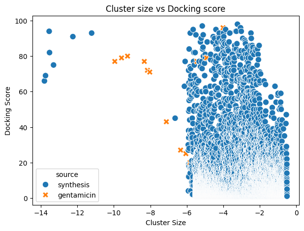
When analysing the output, we observed that seven newly generated molecules displayed top-ranked poses with more favourable docking scores and good-to-excellent cluster sizes compared with the best-performing Gentamicin components.
| index | LigName | docking_score | cluster_size | source |
|---|---|---|---|---|
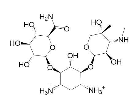
| 0 | AIHDHRVACSMVSS-XAZDVDGLSA-P | -13.81 | 66 | synthesis |
| 1 | ICKHKVBFJNIUOS-SPDZNJQTSA-P | -13.75 | 69 | synthesis |
| 2 | YLQPVHLJFCAXAZ-LDAWGXOASA-P | -13.55 | 94 | synthesis |
| 3 | XCOCCSDVQOFFMD-IECBTLPXSA-P | -13.53 | 82 | synthesis |
| 4 | ZPTFPLASSDISCG-XHHMNFPTSA-P | -13.31 | 75 | synthesis |
| 5 | XCOCCSDVQOFFMD-QZHDWQIISA-P | -12.25 | 91 | synthesis |
| 6 | UDUQYUXNGOGLPX-ARTXYBLXSA-P | -11.22 | 93 | synthesis |
| 7 | Gentamicin_C2b | -9.95 | 77 | gentamicin |
| 8 | Gentamicin_C2a | -9.58 | 79 | gentamicin |
| 9 | Gentamicin_C1a | -9.25 | 80 | gentamicin |
| 10 | Sisomicin | -8.33 | 77 | gentamicin |
| 11 | Gentamicin_C2 | -8.16 | 72 | gentamicin |
| 12 | Gentamicin_C1 | -8.03 | 71 | gentamicin |
| 13 | Gentamicin_X2 | -7.12 | 43 | gentamicin |
| 14 | AIHDHRVACSMVSS-VPNVSPPVSA-P | -6.64 | 45 | synthesis |
| 15 | Gentamicin_B | -6.34 | 27 | gentamicin |
| 16 | PTLBUBLKUHWAIE-XAFKKLOQSA-P | -6.13 | 63 | synthesis |
| 17 | AIHDHRVACSMVSS-ZIUGFXRJSA-P | -6.09 | 77 | synthesis |
| 18 | Gentamicin_A | -6.05 | 25 | gentamicin |
| 19 | NEOAADVDRWNPHK-KZZKPSOFSA-P | -5.92 | 30 | synthesis |
| 20 | KRHWIUYFCZEFNO-BIVBFBQOSA-P | -5.92 | 12 | synthesis |
| 21 | LDSXANXIWFICQQ-RHTYCGIVSA-P | -5.91 | 4 | synthesis |
| 22 | PCYZHRJSYONBMD-MPQDXOOUSA-P | -5.91 | 27 | synthesis |
| 23 | YLQPVHLJFCAXAZ-IKPOJUDMSA-P | -5.9 | 38 | synthesis |
| 24 | WDBBXHFHIONMCT-HQSMMMQGSA-P | -5.9 | 12 | synthesis |
| 25 | ZBYHKGPMAJXMKO-VULWWWRKSA-P | -5.9 | 72 | synthesis |
| 26 | KRHWIUYFCZEFNO-MDJATCENSA-P | -5.89 | 12 | synthesis |
| 27 | KRHWIUYFCZEFNO-VGJLZALASA-P | -5.89 | 34 | synthesis |
| 28 | LDSXANXIWFICQQ-NMOAJELSSA-P | -5.89 | 49 | synthesis |
| 29 | ACLTWIJKUWADKU-FBICMHTBSA-P | -5.89 | 19 | synthesis |
| --- | --- | --- | --- | --- |
| 350 | Garamine | -5.44 | 77 | gentamicin |
| 2537 | 2Deoxystreptamine | -4.91 | 79 | gentamicin |
| 5345 | Garosamine | -4.01 | 96 | gentamicin |
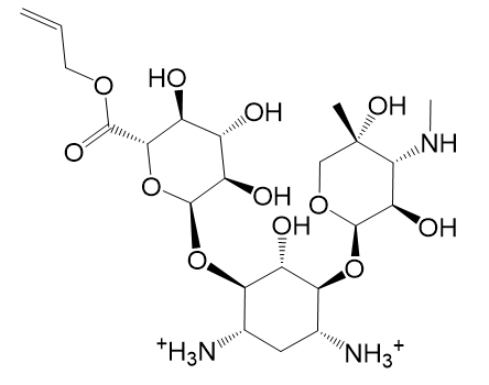
 |  |
|---|---|
| (a) 2D structure AIHDHRVACSMVSS-XAZDVDGLSA-P | (b) 3D structure AIHDHRVACSMVSS-XAZDVDGLSA-P |
 |  |
| (c) 2D structure ICKHKVBFJNIUOS-SPDZNJQTSA-P | (d) 3D structure ICKHKVBFJNIUOS-SPDZNJQTSA-P |
 |  |
| (e) 2D structure YLQPVHLJFCAXAZ-LDAWGXOASA-P | (f) 3D structure YLQPVHLJFCAXAZ-LDAWGXOASA-P |
 |  |
| (g) 2D structure XCOCCSDVQOFFMD-IECBTLPXSA-P | (h) 3D structure XCOCCSDVQOFFMD-IECBTLPXSA-P |
 |  |
| (i) 2D structure ZPTFPLASSDISCG-XHHMNFPTSA-P | (j) 3D structure ZPTFPLASSDISCG-XHHMNFPTSA-P |
 |  |
| (k) 2D structure XCOCCSDVQOFFMD-QZHDWQIISA-P | (l) 3D structure XCOCCSDVQOFFMD-QZHDWQIISA-P |
 |  |
| (m) 2D structure UDUQYUXNGOGLPX-ARTXYBLXSA-P | (n) 3D structure UDUQYUXNGOGLPX-ARTXYBLXSA-P |
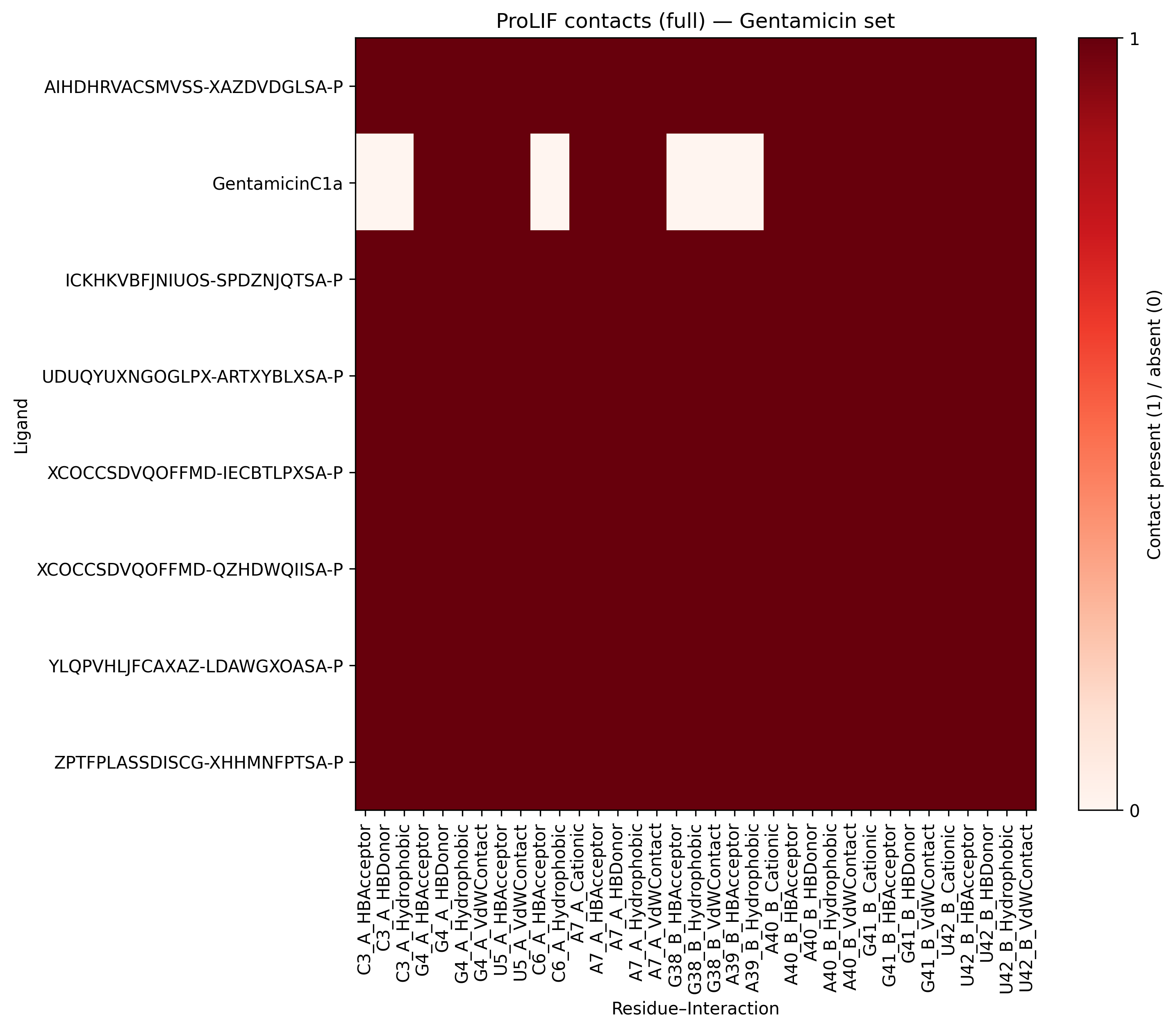
Notably, the ProLIF analysis consistently highlights the canonical interactions established by the Gentamicin C1a reference and other potent natural analogues (Gentamicins C and Sisomicin). However, when exploring the newly proposed hits from the vHTS campaign, additional positive contacts emerge, particularly with residues C3, C6, G38, and G39. These interactions were not previously observed for any of the natural Gentamicin components and may reflect alternative binding strategies or complementary recognition patterns enabled by the novel chemical modifications. Such findings suggest that the synthetic analogues not only reproduce the essential pharmacophoric contacts but also extend the interaction network within the RNA binding site.
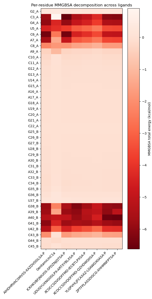
These results are further reinforced by MMGBSA analysis, which demonstrates that the newly identified analogues establish stronger stabilizing energetic contributions with most of the binding site nucleotides compared to the reference Gentamicin C1a. Importantly, while retaining key pharmacophoric interactions, the additional energetic hotspots observed appear to enhance the overall pharmacodynamic profile. Taken together, this dual contact- and energy-based fingerprint supports the hypothesis that these vHTS-derived analogues may represent promising candidates for synthetic prioritization and subsequent biological validation.
Conclusions & Outlook
In this final section we translated the pharmacodynamic insights gleaned from natural Gentamicin congeners into a prospective design–screening cycle. By programmatically assembling ring-I–modified analogues via in silico glycosylation of Garamine with a curated set of 2-tetrahydropyranols, and then benchmarking them under the same docking/ProLIF/MMGBSA pipeline, we identified multiple derivatives with substantially improved docking scores and robust cluster sizes, outperforming the best natural components.
Two converging lines of evidence support their promise:
-
Contact fingerprints (ProLIF): Hits reproduce the canonical A-site contacts (G4, U5, A7, A40, G41, U42) characteristic of potent Gentamicins, and introduce new, consistent contacts (e.g., C3, C6, G38, G39) that were not observed across the natural mixture. This points to expanded recognition rather than a mere mimicry of the reference pose.
-
Energetic fingerprints (MMGBSA): Per-residue decomposition reveals stronger stabilization at both canonical and newly engaged nucleotides, indicating that the added contacts contribute measurably to binding energy after minimization.
Together, these results illustrate how a dual fingerprint strategy (structural contacts + energetic contributions) can discriminate truly promising analogues from look-alikes, and provide a mechanistic rationale for prioritization before synthesis/biology.
Take-home message
This tutorial illustrates how a stepwise workflow—spanning docking, contact fingerprints (ProLIF), and energetic fingerprints (MMGBSA)—can be used not only to rationalize the differential potency of natural congeners but also to guide the design of novel analogues with improved interaction profiles.
Although the case study focused on Gentamicin derivatives, the same strategy is broadly transferable to other drug design projects, regardless of the target class (enzymes, receptors, or nucleic acids) or chemical family. By systematically combining structural and energetic analyses, researchers can:
-
Validate docking protocols against crystallographic references.
-
Dissect pharmacodynamic determinants that explain potency differences.
-
Prioritize synthetic candidates from large enumerated libraries with stronger rationale than docking scores alone.
In this sense, the workflow is best seen not as a Gentamicin-specific pipeline, but as a generalizable platform for virtual screening and rational analogue design, adaptable to any medicinal chemistry campaign aiming to accelerate the discovery of affordable and effective therapeutic agents.
Footnotes
-
Krause, Kevin M., et al. "Aminoglycosides: an overview." Cold Spring Harbor perspectives in medicine 6.6 (2016): a027029. ↩ ↩2 ↩3
-
O’Sullivan, Mary E., et al. "Dissociating antibacterial from ototoxic effects of gentamicin C-subtypes." Proceedings of the National Academy of Sciences 117.51 (2020): 32423-32432. ↩ ↩2 ↩3 ↩4 ↩5
-
François, Boris, et al. "Crystal structures of complexes between aminoglycosides and decoding A site oligonucleotides: role of the number of rings and positive charges in the specific binding leading to miscoding." Nucleic acids research 33.17 (2005): 5677-5690. ↩ ↩2 ↩3 ↩4 ↩5